Essence of Linear Algebra
“There is hardly any theory which is more elementary than linear algebra, in spite of the fact that generations of professors and textbook writers have obscured its simplicity by preposterous calculations with matrixes.”
1. What vector is
three ideas:
physics students: arrows pointing in space length and directions
computer science students: ordered lists of numbers
mathematicians: a vector can be anything (abstract)
vector addition and multiplication by numbers
\[\vec{a}+\vec b \qquad \vec a\vec b\]Each vector represents a certain movement, a step with a certain distance and direction in space. If you take a step along the first vector, then take a step in the direction and distance by the second vector, the over all affect is just the same as if you move along the sum of those two vectors to start with.
\[\left[\begin{matrix} x_1\\x_2 \end{matrix}\right] + \left[\begin{matrix} y_1\\y_2 \end{matrix}\right] = \left[\begin{matrix} x_1+y_1\\x_2+y_2 \end{matrix}\right]\]Throughout linear algebra, one of the main things that numbers do is scale vectors. In the conception of vectors as lists of numbers, multiplying a given vector by a scalar means multiplying each one of those components by that scalar.
\[2 \times \left[\begin{matrix} x_1\\x_2 \end{matrix}\right] = \left[\begin{matrix} 2x_1\\2x_2 \end{matrix}\right]\]The usefulness of linear algebra has less to do with either one of these views, than it does with the ability to translate back and forth between them. It gives the data analyst a nice way to conceptualize many lists of numbers in a visual way, which can seriously clarify patterns in data, and give a global view of what certain operations do. And on the flip side, it gives people like physicists and computer graphics programmers a language to describe space and the manipulation of space using numbers that can be crunched and run through a computer.
2. Linear combinations, span, and bases
vector coordinates
Think of each coordinate as a vector, and think about how each one stretches or squishes vectors. In two dimension coordinate systems, here are two special vectors: $\hat i$ and $\hat j$. Then we have, for example:
\[\left[\begin{matrix} x_1\\x_2 \end{matrix}\right] = x_1 \hat i+ x_2 \hat j\]$\hat i$ and $\hat j$ are the “basis vectors” of the $xy$ coordinate system. We could choose different basis vectors, and gotten a completely reasonable, new coordinate systems. “Linear combination” of $\vec v$ and $\vec w$:
\[a \vec v + b \vec w\]About the “linear”, if you fix one of those scalars and let the other change its value freely, the tip of the result vector draw a straight line.
The “span” of $\vec v $ and $\vec w$ is the set of all their linear combinations. The span of most pairs of 2-D vectors is all vectors of 2-D space. But when they line up, their span is all vectors whose tip sits on a certain line.
vectors VS points
linearly dependent and linearly independent
\[\begin{gather*} \vec u=a \vec v + b \vec w\\ \vec u \neq a \vec v + b \vec w \end{gather*} \\(For\ all\ value\ of\ a\ and\ b)\]The basis of a vector space is a set of linearly independent vectors that span the full space.
3. Matrixes as linear transformations
linear transformation: takes a vector input and has a vector output
Image watching every possible input vector move over to its corresponding output vector.
-
Lines remain lines.
-
Origin remains fixed.
It turns out that you only need to record where the two basis vectors— $\hat i$ and $\hat j$ — each land, and everything else will follow from that.
For example:
\[\vec v= \left[ \begin{matrix} x \\ y \end{matrix} \right] =x \hat i + y\hat j\] \[\\Transformed\ \hat i= \left[ \begin{matrix} -1 \\ 2 \end{matrix} \right] \qquad Transformed\ \hat j= \left[ \begin{matrix} 3 \\ 0 \end{matrix} \right]\] \[\\Transformed\ \vec v= x\ (Transformed\ \hat i) + y\ (Transformed\ \hat j)\\ \qquad \qquad= x \times \left[ \begin{matrix} -1 \\ 2 \end{matrix} \right] + y \times\left[ \begin{matrix} 3 \\ 0 \end{matrix} \right] = \left[ \begin{matrix} -x + 3y \\ 2x \end{matrix} \right]\]A two dimensional linear transformation is completely described by just four numbers: the two coordinates of $\hat i$ and $\hat j$ after transforming. It’s common to package these coordinates into a 2-by-2 grid of numbers,called a 2-by-2 matrix. Matrix here is just a way of packaging the information needed to describe a linear transformation.
\[M = \left[\begin{matrix} a & b\\ c & d \end{matrix}\right ]\]Thinking of the idea before, we have:
\[\left[\begin{matrix} a & b \\ c & d \end{matrix}\right] \left[\begin{matrix} x \\ y \end{matrix}\right] =x \left[\begin{matrix} a \\ c \end{matrix}\right] +y \left[\begin{matrix} b \\ d \end{matrix}\right] = \left[\begin{matrix} ax+by \\ cx+dy \end{matrix}\right]\]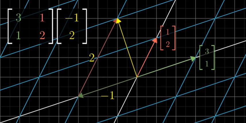
Technically, the definition of “linear” is as follows: A trans formation L is linear if it satisfies these two properties:
\[\begin{gather*} L(\vec v + \vec w) = L(\vec v) + L(\vec w) \tag{1}\\ \end{gather*}\] \[L(c\vec v) = cL(\vec v)\tag{2}\]4. Matrix multiplication as compositions
Describe the effects of applying one transformation and then another. This new linear transformation can be called the “composition” of the two separate transformations we applied.
For example, first rotation then shear:
\[\left [ \begin{matrix} 1 & 1\\ 0 & 1 \end {matrix} \right ]_{Shear} \times \left ( \left [ \begin{matrix} 0 & -1\\ 1 & 0 \end {matrix} \right ]_{Rotation} \times \left [ \begin{matrix} x\\ y \end {matrix} \right ] \right ) = \left [ \begin{matrix} 1 & -1\\ 1 & 0 \end {matrix} \right ]_{Composition} \times \left [ \begin{matrix} x\\ y \end {matrix} \right ]\]Multiplying two matrices like this has the geometric meaning of applying one transformation then another.
Read right to left!
\[M_1 M_2 \neq M_2 M_1\]To proof that $(AB)C=A(BC)$, we just need to find that the calculate order hasn’t been changed.
5. Linear transformations in three dimensions
There are three standard basis vectors that we typically use: $\vec x, \vec y\ and\ \vec z $. This gives a matrix that completely describes the transformation using only nine numbers.
\[\vec v= \left[ \begin{matrix} x & y & z \end{matrix} \right] ^T =x \hat i + y \hat j + z \hat k\]For example, as a linear transformation, we have:
\[\left[\begin{matrix} 0 & 1 & 2 \\ 3 & 4 & 5 \\ 6 & 7 & 8 \end{matrix}\right] \left[\begin{matrix} x \\ y \\ z \end{matrix}\right] =x \left[\begin{matrix} 0 \\ 3 \\ 6 \end{matrix}\right] +y \left[\begin{matrix} 1 \\ 4 \\ 7 \end{matrix}\right] +z \left[\begin{matrix} 2 \\ 5 \\ 8 \end{matrix}\right]\]Multiplying two matrices is also similar.
6. The determinant
Think of the linear transformations, you might notice how some of them seemed to stretch space out, while others squish it on in. One thing that turns out to be pretty useful for understanding one of these transformations is to measure exactly how much it stretches or squishes things.
This very special scaling factor-the factor by which a linear transformation changes any area, is called the determinant of that transformation.
\[det \left ( \left [ \begin{matrix} 3 & 2 \\ 0 & 2 \end {matrix} \right ] \right) =6\]The determinant of a 2-D transformation is 0, if it squishes all of the space on to a line, or even onto a single point, since then, the area of any region would become 0.
Negative number?
Any transformations that do this are invert the orientation of space.
Here is the way to calculate the 2-D determinants:
\[det \left ( \left [ \begin{matrix} a & b \\ c & d \end {matrix} \right ] \right) = (a+b)(c+d)-ac-bd-2bc = ad-bc\]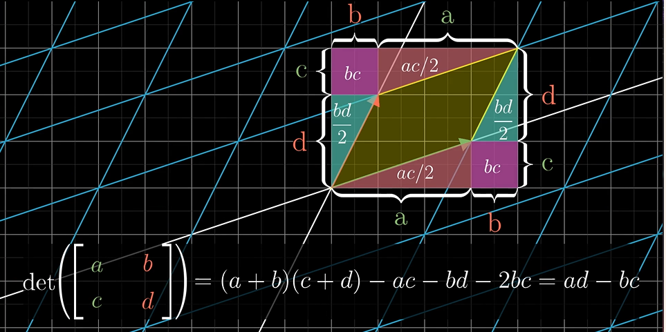
About the more dimensions determinants, we have, for example:
\[det \left ( \left [ \begin{matrix} a & b & c \\ d & e & f \\ g & h & i \end {matrix} \right ] \right) = a\ det \left ( \left [ \begin{matrix} e & f \\ h & i \end {matrix} \right ] \right) - b\ det \left ( \left [ \begin{matrix} d & f \\ g & i \end {matrix} \right ] \right) + c\ det \left ( \left [ \begin{matrix} d & e \\ g & h \end {matrix} \right ] \right)\]It’s easy for us using this idea to proof: $det(M_1M_2)=det(M_1)det(M_2)$
7. Inverse matrixes, column space and null space
Systems of equations: linear system equations
\[\begin {gather} 2x + 5y + 3z = -3\\ 4x + 0y + 8z = 0 \\ 1x + 3y + 0z = 2 \end{gather} \\ \quad \Rightarrow \left [ \begin{matrix} 2 & 5 & 3 \\ 4 & 0 & 8 \\ 1 & 3 & 0 \end {matrix} \right ] \left [ \begin{matrix} x \\ y \\ z \end {matrix} \right ] =\left [ \begin{matrix} -3 \\ 0 \\ 2 \end {matrix} \right ]\] \[A \vec x= \vec v\]The matrix $A$ corresponds with some linear transformation, so solving $A \vec x=\vec v$ means we’re looking for a vector $\vec x$, which after applying the transformation lands on $\vec v$.
-
$det(A)\neq 0$
In this case, there will always be one and only one vector that lands on $\vec v$, and you can find it by playing the transformation in reverse. When you play the transformation in reverse, it actually corresponds to a separate linear transformation, commonly called “the inverse of $A$”, denoted $A^{-1}$.
In general, $A^{-1}$ is the unique transformation with the property that if you first apply $A$, then follow it with the transformation $A$ inverse, you end back where you started, which means you get the transformation that does nothing.
-
$ det(A)=0$
When the determinant is 0, and the transformation of this system of equations squishes space into a smaller dimension, there is no inverse. You can not “unsquish” a line to turn it into a plane.
Rank: the number of dimensions in the output (the number of dimensions in column space)
Column space: set of all possible outputs $A \vec v$
Full rank
The vector $[0\quad 0]^T$ is always in the column space.
Null space or kernel
8. Nonsquare matrices
transformations between dimensions, for example:
\[A = \left [ \begin{matrix} 2 & 0 \\ -1 & 1 \\ -2 & 1 \end {matrix} \right ]\]The column space of this matrix, the place where all the vectors land, is a 2-D plane slicing through the origin of 3-D space. But the matrix is still full rank. It has the geometric interpretation of mapping two dimensions to three dimensions.
9. Dot products and duality
The dot product between two vectors of the same dimension, for example:
\[\left [ \begin{matrix} 4 \\ 1 \end {matrix} \right ] \cdot \left [ \begin{matrix} 2 \\ -1 \end {matrix} \right ] = 4\cdot 2 + 1\cdot -1 = 7\]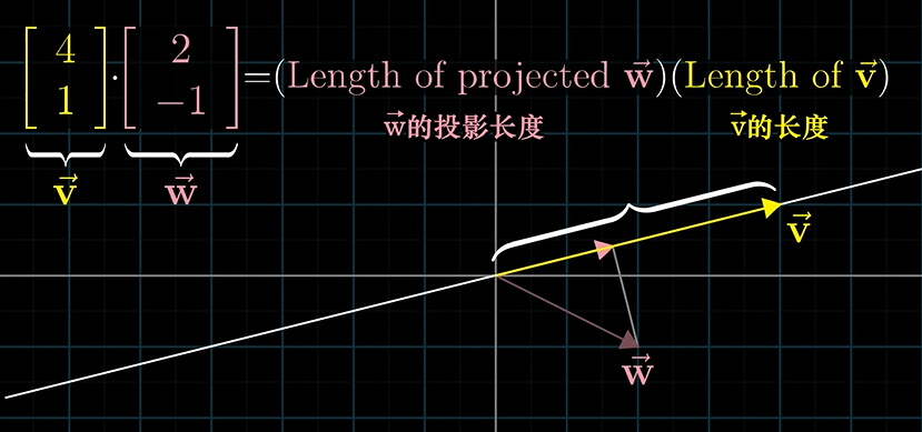
If you take a line of evenly spaced dots and apply a transformation, a linear transformation will keep those dots evenly spaced once they land in the output space, which is the number line. And we also have, for example, $A=[4\quad 1]$ as a $2 \times 1\ matrices$ to describe a 2-D to 1-D linear transformation, we have:
\[Result = [4\quad 1] \times \left [ \begin{matrix} a \\ b \end {matrix} \right ] = 4a + b\]So, here is a question:
\[1 \times 2 \ matrices\ \Longleftrightarrow\ 2D\ vectors \ ?\]Think of a number line in a 2-D space, $\hat i$, $\hat j$ and $\hat u$ are all unit vectors
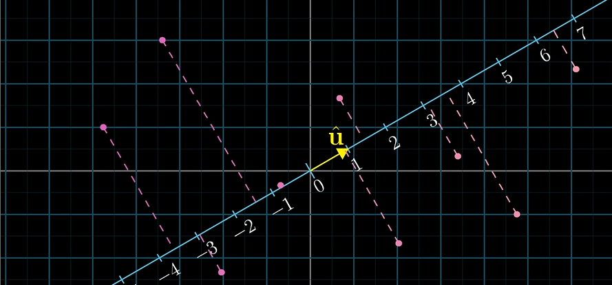
Then we find the $1\times2\ matrix\ B$ to describe the transformation:
\[B=[\hat u_x\quad \hat u_y]\]$\hat u_x$ means where the $\hat i$ lands on the number line, and $\hat u_y$ is similar. So the entries of the $1\times 2$ matrix describing the projection transformation are going to be the coordinates of $\hat u$. This is why taking a dot product with a unit vector can be interpreted as projecting a vector onto the span of that unit vector and taking the length. Non-unit vectors are similar.
\[[u_x\quad u_y] \left [ \begin{matrix} x \\ y \end {matrix} \right ] = u_x x + u_y y\] \[\left [ \begin{matrix} u_x \\ u_y \end {matrix} \right ] \cdot \left [ \begin{matrix} x \\ y \end {matrix} \right ] = u_x x + u_y y\]Duality
Doting two vectors together is a way to translate one of them into the world of transformations. Think the vector as the physical embodiment of a linear transformation.
10. Standard introduction of cross products
Order matters
\[\vec v \times \vec w = - \vec w \times \vec v\]In fact, the order of your basis vectors is what defines orientation.

Here is a way using the determinant to calculate the cross products:
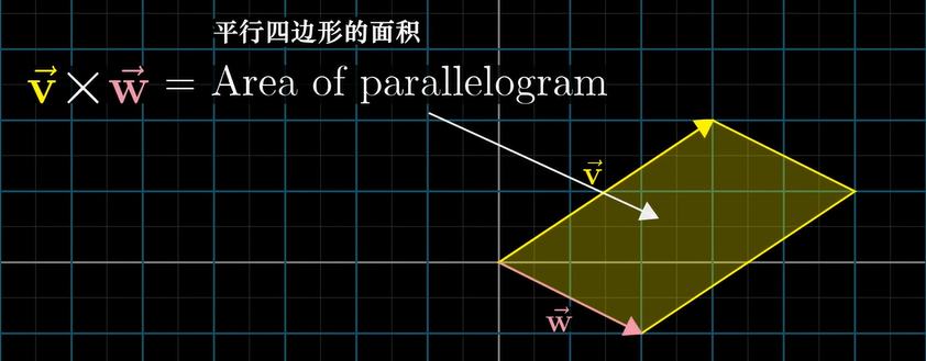
\[\vec v \times \vec w = det \left( \left [ \begin{matrix} \vec v & \vec w \end {matrix} \right] \right)\]But you should remember that the cross product is not a number, it’s a vector. This new vector’s length will be the area of that parallelogram, and the direction of the new vector is going to be perpendicular to the parallelogram, and this vector’s direction obey the right hand rule.
In general, we have:
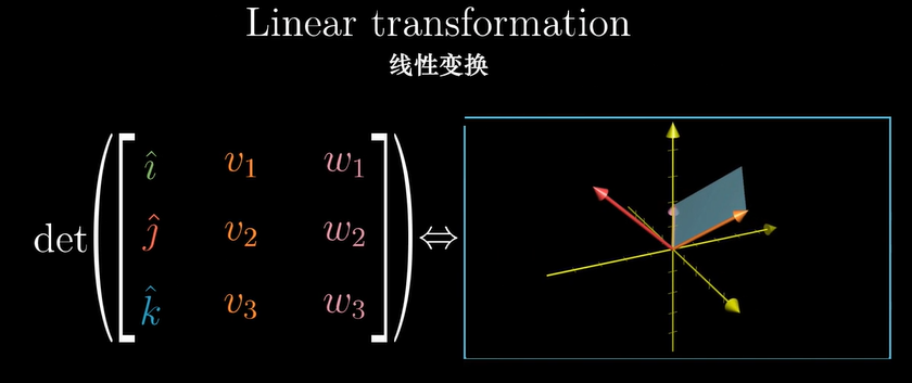
\[\vec v \times \vec w = \vec p\\ \left [ \begin{matrix} v_1 \\ v_2 \\ v_3 \end {matrix} \right] \times \left [ \begin{matrix} w_1 \\ w_2 \\ w_3 \end {matrix} \right] = det \left( \left [ \begin{matrix} \hat i & v_1 & w_1 \\ \hat j & v_2 & w_2 \\ \hat k & v_3 & w_3 \end {matrix} \right] \right)\]11. Cross products in the light of linear transformations
- Define a 3D-to-1D linear transformation in terms of $\vec v$ and $\vec w$.
- Find its dual vector
- Show that this dual is $\vec v \times \vec w$
Think of a $3 \times 3$ matrix, consider that first vector $\vec u$ to be a variable, say with variable entries $[x\quad y\quad z]^T$, while $\vec v$ and $\vec w$ remain fixed. Then we have a function from 3D to 1D. You input some vector $[x\quad y\quad z]^T$ and you get out a number by taking the determinant of a matrix. Geometrically, the meaning of this function is that for any input vector $[x\quad y\quad z]^T$, you consider the parallelepiped defined by this vector, $\vec v$ and $\vec w$, then you return its volume, with the plus or minus sign depending on orientations.
\[f\left( \left [ \begin{matrix} x \\ y \\ z \end {matrix} \right] \right) = det \left( \left [ \begin{matrix} x & v_1 & w_1 \\ y & v_2 & w_2 \\ z & v_3 & w_3 \end {matrix} \right] \right)\]This function is linear. Then we have:
\[\left [ \begin{matrix} p_1 \\ p_2 \\ p_3 \end {matrix} \right] \cdot \left [ \begin{matrix} x \\ y \\ z \end {matrix} \right] = det \left( \left [ \begin{matrix} x & v_1 & w_1 \\ y & v_2 & w_2 \\ z & v_3 & w_3 \end {matrix} \right] \right)\]We just need to find what vector $\vec p$ has the property that when you take a dot product between $\vec p$ and some vector $[x\quad y\quad z]^T$, it gives in the same result as plugging in $[x\quad y\quad z]^T$ to the first column of the matrix.
Think of the geometric interpretation of dot products:
\[\vec p \cdot \left [ \begin{matrix} x \\ y \\ z \end {matrix} \right] = (Length\ of\ projection) \times (Length\ of\ \vec p)\]So the vector $\vec p$ must be perpendicular to $\vec v$ and $\vec w$, with a length equal to the area of the parallelogram spanned out by those two vectors.
12. Change of basis
Think the two basic vectors as encapsulating all of the implicit assumptions of our coordinate system, like the first coordinate, the second coordinate and the unit of distance. Anyway to translate between vectors and sets of numbers is called a coordinate system, and the two special vectors, $\hat i$ and $\hat j$, are called the basis vectors of our standard coordinate system.
Using a different set of basis vectors
So how do we translate between coordinate systems?
\[A \left [ \begin{matrix} x_j \\ y_j \end {matrix} \right]_{Vectors\ in\ J\ coordinates } = \left [ \begin{matrix} x_o \\ y_o \end {matrix} \right]_{Vectors\ in\ O\ coordinates }\]In which, $A$ means the basis vectors of J coordinates written in O coordinates, and the inverse matrix does the opposite:
\[\left [ \begin{matrix} x_j \\ y_j \end {matrix} \right]_{Vectors\ in\ J\ coordinates } = A^{-1} \left [ \begin{matrix} x_o \\ y_o \end {matrix} \right]_{Vectors\ in\ O\ coordinates }\]So think of a linear transformation $M$ on O coordinates, if we want to use it in J coordinates, we have:
\[\left [ \begin{matrix} x'_j \\ y'_j \end {matrix} \right]_{New\ ectors\ in\ J\ coordinates } = A^{-1}MA \left [ \begin{matrix} x_j \\ y_j \end {matrix} \right]_{Vectors\ in\ J\ coordinates }\]An expression like $A^{-1}MA$ suggests a mathematical sort of empathy.
13. Eigenvectors and eigenvalues
Think of a linear transformation $M$ in 2D space, most vectors are going to get knocked off their span during the transformation, but some special vectors do remain on their own span, meaning the effect that the matrix has on such a vector is just to stretch it or squish it, like a scalar.
These special vectors are called the “eigenvectors” of the transformation, and each eigenvector has associated with it, what’s called an “eigenvalue”, which is just the factor by which it stretched or squashed during the transformation. For example, the eigenvector of a 3D rotation matrix which has eigenvalue as 1 is the vector to describe the axis of the rotation.
\[A\vec v = \lambda \vec v\]We want a nonzero solution for $\vec v$ satisfy the follows:
\[(A - \lambda I) \vec v = \vec 0\]which means:
\[det(A - \lambda I)= 0\]Eigenbasis
If both basis vectors are eigenvectors, writing their new coordinates as the columns of a matrix, then we will find that the eigenvalues of the two vectors sit on the diagonal of our matrix and every other entry is 0. This is a diagonal matrix. It is easier to compute what will happen if you multiply this matrix by itself a whole bunch of times.
If your transformation has a lot of eigenvectors, enough so that you can choose a set that spans the full space, then you can change your coordinates system so that these eigenvectors are your basis vectors. The whole point of doing this with eigenvectors is that this new matrix is guaranteed to be diagonal with its corresponding eigenvalues down that diagonal.
However, a shear, for example, does not have enough eigenvectors to span the full space.
Here is a puzzle, taking the following matrix:
\[A = \left [ \begin {matrix} 0 & 1 \\ 1 & 1 \end {matrix} \right ]\]Start computing its first few powers by hand: $A^2$, $A^3$, etc. What pattern do you see? Can you explain why this pattern shows up? This might make you curious to know if there’s an efficient way to compute arbitrary powers of this matrix, $A^n$ for any number n.
Given that two eigenvectors of this matrix are:
\[\vec v_1= \left [ \begin{matrix} 2 \\ 1+\sqrt{5} \end {matrix} \right] \qquad \vec v_2 \left [ \begin{matrix} 2 \\ 1-\sqrt{5} \end {matrix} \right]\]See if you can figure out a way to compute $A^n$ by first changing to an eigenbasis, compute the new representation of $A^n$ in that basis, then converting back to our standard basis. What does this formula tell you?
14. Abstract vector spaces
Determinant and eigenvectors don’t care about the coordinate system. The determinant tells you how much a transformation scales areas, and eigenvectors are the ones that stay on their own span during a transformation. You can freely change your coordinate system without changing the underlying values of either one.
Think about the function.
Consider the derivative as a linear transformation (linear operator). What does it mean for a transformation of functions to be linear? Linear transformation preserve addition and scalar multiplication.
\[Activity:\quad L(\vec v + \vec w) = L(\vec v) + L(\vec w)\\\] \[Scaling:\quad L(c\vec v) = cL(\vec v)\]A linear transformation is completely described by where it takes the basis vectors. Since any vector can be expressed by scaling and adding the basis vectors in some way, finding the transformed version of a vector comes down to scaling and adding the transformed versions of the basis vectors in that same way. This is as true for functions as it for arrows.
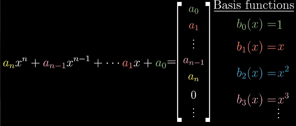
For example, we have our current space: all polynomials. The first thing we need to do is giving coordinates to this space, which requires choosing a basis. It’s pretty natural to choose pure powers of $x$ as the basis functions, which are infinite.
In this coordinate system, the derivative is described with an infinite matrix, that’s mostly full of zeros, but which has the positive integers counting down on this offset diagonal. For example:
\[\frac{d}{dx} (1x^3 + 5x^2 + 4x +5) = 3x^2 + 10x + 4\] \[\left [ \begin {matrix} 0 & 1 & 0 & 0 & \cdots\\ 0 & 0 & 2 & 0 & \cdots\\ 0 & 0 & 0 & 3 & \cdots\\ 0 & 0 & 0 & 0 & \cdots\\ \vdots & \vdots & \vdots & \vdots & \ddots \end {matrix} \right ] \left [ \begin {matrix} 5 \\ 4 \\ 5 \\ 1 \\ \vdots \end {matrix} \right ] = \left [ \begin {matrix} 1\cdot 4 \\ 2\cdot 5 \\ 3\cdot 1 \\ 0 \\ \vdots \end {matrix} \right ]\]| Linear algebra concepts | Alternate names when applied to functions |
|---|---|
| Linear transformations | Linear operators |
| Dot products | Inner products |
| Eigenvectors | Eigenfunctions |
Vector spaces
Rules for vectors addition and scaling:
- $ \vec u + (\vec v + \vec w) = (\vec u + \vec v) + \vec w$
- $\vec v + \vec w = \vec w + \vec v$
- There is a vector $\vec 0$ such that $\vec 0 + \vec v = \vec v$ for all $\vec v$
- For every vector $\vec v$ there is a vector $-\vec v$ so that $\vec v+(-\vec v)=0$
- $a(b\vec v)=(ab)\vec v$
- $1\vec v=\vec v$
- $a(\vec v+\vec w)=a\vec v+a\vec w$
- $(a+b)\vec v = a\vec v + b\vec v$