Here is the first half part of the notes for CS231n: Convolutional Neural Networks for Visual Recognition from Stanford University. The official notes are published on the course website. Since they only public the videos in 2017, which is a relatively elder version compared with the recent development of computer vision, I also recommend IN2364: Advanced Deep Learning for Computer vision, Spring 2020 from Technical University of Munich and EECS 498-007 / 598-005 Deep Learning for Computer Vision from University of Michigan as supplementary materials.

Deep Learning for Computer Vision

1. Course Introduction

Visual Data: Dark matter of the Internet

The field of computer vision is truly an interdisciplinary field, and it touches on many different areas of science and engineer and technology.

The history of vision 1600s the Renaissance period of time camera obscura

1959 Hubel & Wiesel the visual processing mechanism

1970 David Marr Vision

• Input images: Perceived intensities
• Primal Sketch: Zero crossings, blobs, edges, bars, ends, virtual lines, groups, curves boundaries
• 2.5D Sketch: Local surface orientation and discontinuities in depth and in surface orientation
• 3-D Model Representation: 3-D models hierarchically organized in terms of surface and volumetric primitives

1979 Brooks & Binford Generalized Cylinder

1973 Fischler and Elschlager Pictorial Structure

• Object s composed of simple geometric primitives.

1987 David Lowe Try to recognize razors by constructing lines and edges.

1997 Shi & Malik Normalized Cut

1999 David Lowe “SIFT” & Object Recognition

2001 Viola & Jones Face Detection

2006 Lazebnik, Schmid & Ponce Spatial Pyramid Matching

2005 Dalal& Trigas Histogram of Gradients

2009 Felzenswalb, McAllester, Ramanan Deformable Part Model

CS231-n overview

CS231-n focuses on one of the most important problems of visual recognition-image classification. There is a number of visual recognition problems that are related to image classification, such as object detection, image captioning.

Convolutional Neural Networks (CNN) have become an important tool for object recognition.

2. Image Classification

Image Classification: A core task in Computer Vision

An image is just a big grid of numbers between [0,255].

The problem and challenge

• Semantic gap
• Viewpoint variation
• Illumination
• Deformation
• Occlusion
• Background Clutter
• Interclass variation

An image classifier

1
2
3
def classify_image(image):
    # Some magic here?
    return class_label

There is no obvious way to hard-code the algorithm for recognizing a cat or other classes.

We want to come up with some algorithm or some method for these recognition tasks, which scales much more naturally to all the variety of objects in the world.

Data-Driven Approach

1. Collect a dataset of images and labels
2. Use machine learning to train a classifier
3. Evaluate the classifier on new images

1
2
3
4
5
6
7
def train(image, labels):
    # Machine learning!
    return model

def predict(model, test_images):
    # Use model to predict labels
    return test_labels

First classifier: Nearest Neighbor

1. During the training, it just need to memorize all the data and labels.
2. And then predict the label of the most similar training image.

Use the distance metric to compare images.

With N examples, the training is $O(1)$ and predicting is $O(N)$. This is bad, because we want classifiers that are fast at prediction; slow for training is OK.

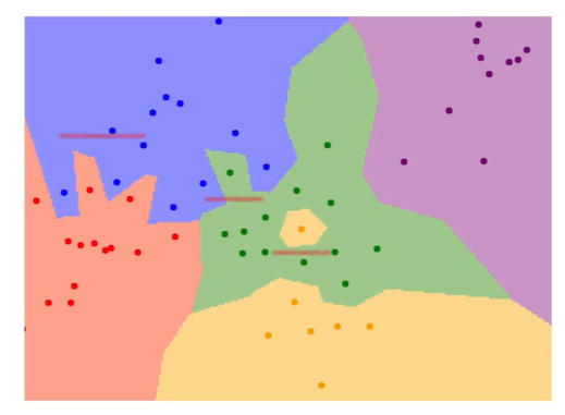
K-nearest neighbors

Instead of copying label from nearest neighbor, take majority vote from K closest points.

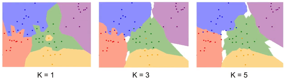
The K can smooth our boundaries and lead to better results.

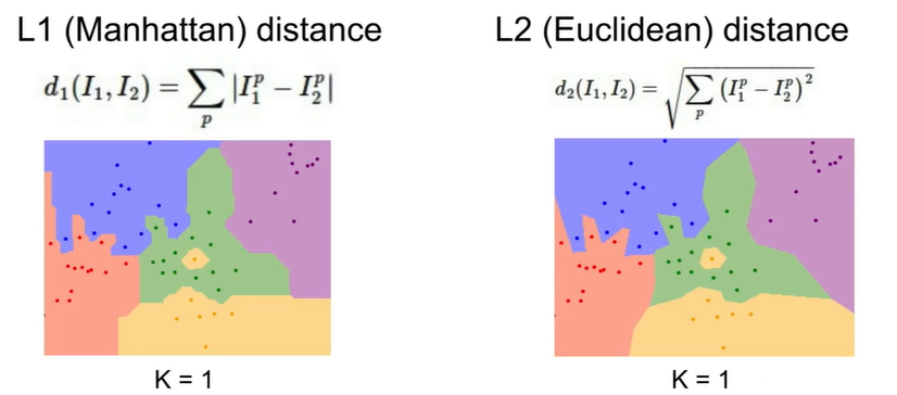
Distance Metric:

L1(Manhattan) distance: $d_1 (I_1,I_2) = \sum_p {|I_1^p - I_2^p|}$

L2(Euclidean) distance: $d_2 (I_1,I_2) = \sqrt{\sum_p (I_1^p - I_2^p)^2}$

Different distance metrics make different assumptions about the underlying geometry or topology that you’d expect in the space.

Each points in the two figures have the same distances to the original point. The first one use L1 distance and the second one using L2 distance.

The L1 distance depends on the choice of your coordinate frame. So if you rotate the coordinate frame that would actually change the L1 distance between the points. Whereas change the frame that in the L2 distance doesn’t matter.

You can use this algorithm on many different types of data.

Hyperparameters

What is the best value of k to use? What is the best distance to use? These are hyperparameters: choices about the algorithm that we set rather than learn. This is very problem-dependent because we must try them all out and see what works best.

Setting hyperparameters

Split data into train, validation and test, choose hyperparameters on validation and evaluate on test. Split data into folds, try each fold as validation and average the results. This is useful for small datasets, but not used too frequently in deep learning. Here is an example of 5-fold cross-validation for the value of K.

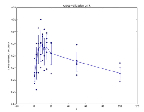
Each point is a single outcome, the line goes through the mean, and the bars indicated the standard deviation.

k-Nearest Neighbor on images never used.

• Very slow at test time.
• Distance metrics on pixels are not informative.
• Curse of dimensionality

Linear Classification

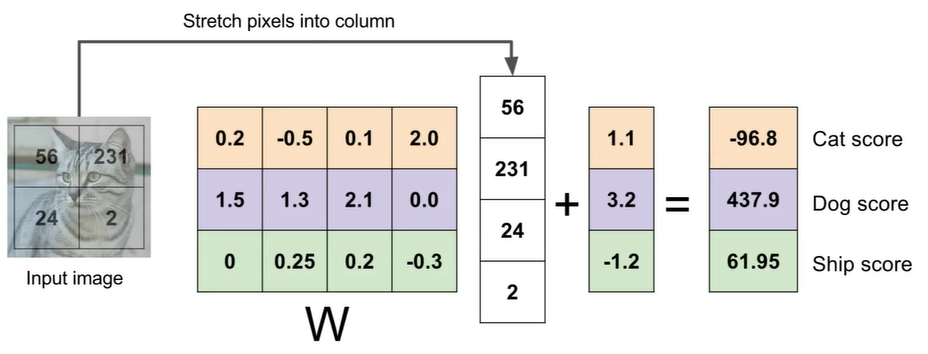
Parametric Approach: Linear Classifier

X is the image input, such as an array of $32 \times 32 \times 3$ numbers (3072 in total)

W are parameters or weights

Output is 10 numbers giving class scores.

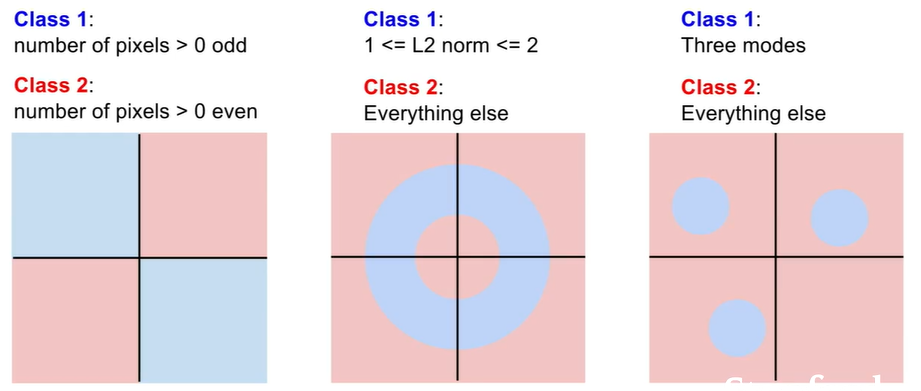
Hard cases for a linear classifier

So how to choose the right W?

3. Loss Functions and Optimization

Linear Classifier

1. Define a loss function that quantifies our unhappiness with the scores across the train data.
2. Come up with a way of efficiently finding the parameters that minimize the loss function.(Optimization)

A loss function tells how good our current classifier is.

Given a dataset of examples:

Where $x_i$ is image and $y_i$ is label.

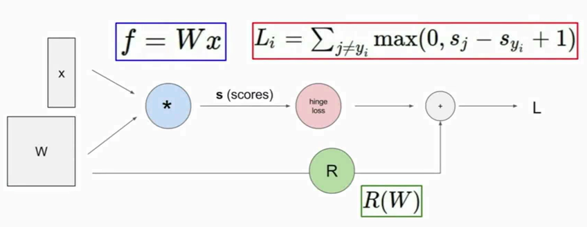
Loss over the dataset is a sum of loss over examples:

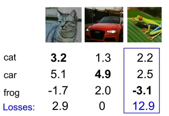
And we called the multiclass SVM loss the “Hinge loss”.

where $y_1$ is the category of the ground truth label for the example, so the $s_{y_1}$ corresponds to the score of the true class for the i-th example in the training set.

The code to calculate the loss function using numpy.

1
2
3
4
5
6
def L_i_vectorized(x, y, W):
    scores = W.dot(x)
    margins = np.maximum(0, scores - scores[y] + 1)
    margins[y] = 0
    loss_i = np.sum(margins)
    return loss_i

Using the multiclass SVM loss, we have:

E.g. Suppose that we found a W such that $L=0$. Is this $W$ unique? No!

The concept of regularization

Model should be “simple”, so it works on test data. We can add another term on the loss function which encourages the model to somehow pick a simpler W, where the concept of simple kind of depends on the task and the model.

• $L_2$ regularization $R(W)=\sum_k\sum_lW_{k,l}^2$
• $L_1$ regularization $R(W)=\sum_k\sum_l|W_{k,l}|$
• Elastic net ($L_1+L_2$) $R(W)=\sum_k\sum_l\beta W_{k,l}^2+ |W_{k,l}|$

Softmax Classifier (Multinomial Logistic Regression)

Want tot maximize the log likelihood, or (for a loss function) to minimize the negative log likelihood of the correct class:

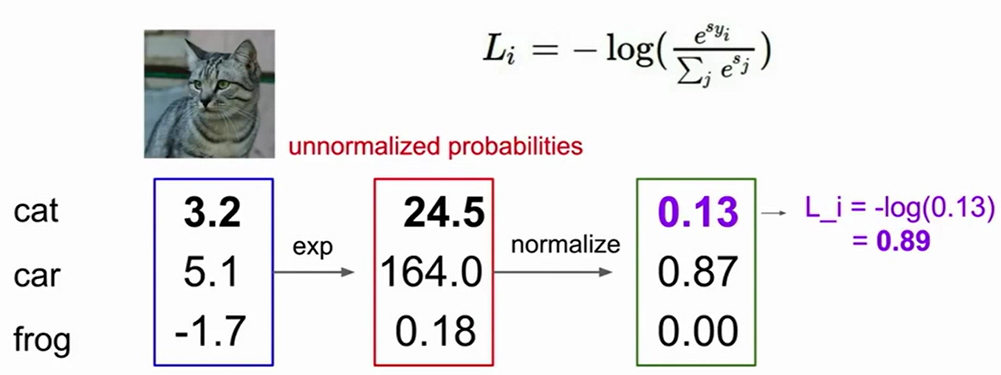
The only thing that the SVM loss cared about was getting that correct score to be greater than a margin above the incorrect scores. But now the softmax loss is actually quite different in this respect. The softmax loss actually always wants to drive that probability mass all the way to one. So the softmax class always try to continually to improve every single data point to get better and better.

Optimization

In practice, we tend to use various types of iterative methods, where we start with some solutions and then gradually improve it over time.

Random Research $\times$

Follow the slope

In one dimension, the derivative of a function:

In multiple dimensions, the gradient is the vector of partial derivatives along each dimension. The slope in any direction is the dot product of the direction with the gradient. The direction of steepest descent is the negative gradient.

Numerical gradient: approximate, slow, easy to write

Analytic gradient: exact, fast, error-prone

In practice, we always use analytic gradient, but check implementation with numerical gradient. This is called a gradient check.

1
2
3
4
# Vanilla Gradient Descent
while True:
    weights_grad = evaluate_gradient(loss_fun, data, weights)
    weights += -step_size * weights_grad     # perform parameter update

The step size is a very significant super-parameter, which is often the first thing we try to set.

Stochastic Gradient Descent (SGD)

Full sum is expensive when N is large, so we often approximate sum using a mini-batch of examples, and 32, 64, 128 ($2^n$) is common.

1
2
3
4
5
# Vanilla Minibatch Gradient Descent
while True:
    data_batch = sample_train_data(data, 256) # sample 256 examples
    weights_grad = evaluate_gradient(loss_fun, data_batch, weights)
    weights += -step_size * weights_grad     # perform parameter update

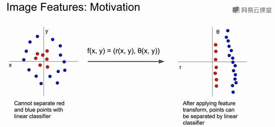
Image Features

The feature representation of the image will be fed into the linear classifier rather than feeding the raw pixels themselves into the classifier.

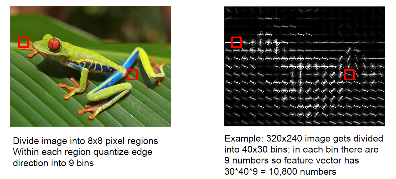
Example: Histogram of Oriented Gradients (HoG)

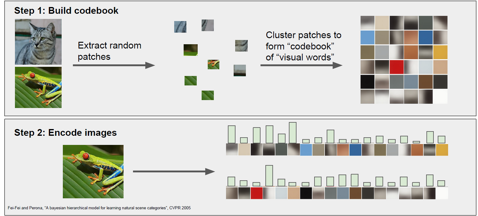
Example: Bag of words

Defined the vocabulary vision words and encode images.

4. Backpropagation and Neural Networks

Here is the way to compute the analytic gradient for arbitrary complex functions.

Computational graphs

Computational graph is that we can use this kind of graph in order to represent any function, where the nodes of the graph are steps of computation that we go through.

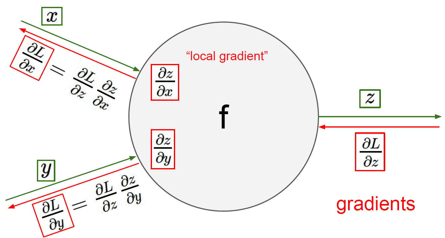
Once we can express a function using a computational graph, then we can use the technique that we call back-propagation, which is going to recursively use the chain rule in order to compute the gradient with respect to every variable in the computational graph.

At each node, we had its local input that are connected to this node, and then we also have the output that is directly outputted from this code.

We can also group some nodes together as long as we can write down the local gradient for that node. For example, as the sigmoid function, we have:

What’s the max gate look like?

• add gate: gradient distributor
• max gate: gradient router
• multiply gate : gradient switcher

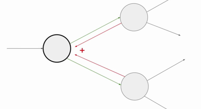
Gradients add at branches.

Gradients for vectorized code

A vectorized example:

Always check, the gradient with respect to a variable should have the same shape as the variable, and each element of the gradient is how much of the particular element affect our final output of the function.

Modularized implementation: forward/backward API

1
2
3
4
5
6
7
8
9
10
11
12
class ComputationalGraph(object):
    # ...
    def forward(inputs):
        # 1. pass inputs to the gates...
        # 2. forward the computational graph:
        for gate in self.graph.nodes_topologically_sorted():
            gate.forward()
        return loss # the final gate in the graph output the loss
    def backward():
        for gate in reversed(self.graph.nodes_topologically_sorted()):
            gate.backward() # little piece of backprop (chain rule applied)
        return inputs_gradients

1
2
3
4
5
6
7
8
9
class MultiplyGate(object):
    def forward(x,y):
        z = x * y
        self.x = x # must keep these around!
        self.y = y
        return z
    def backward(dz):
        dx = self.y * dz # dz/dx * dL/dz
        dy = self.x * dz # dz/dy * dL/dz

Example: Caffe layers

Neural Networks

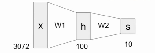
• Before: Linear score function: $f=Wx$
• Now: 2-layer Neural Network: $f=W_2max(0,W_1x)$
• Or more layers

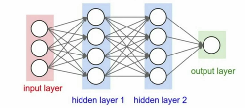
Neural networks are a class of functions where we have simpler functions that are stacked on top of each other, and we stack them in a hierarchical way in order to make up a more complex non-linear function.

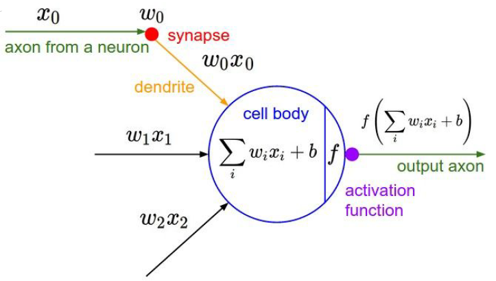
Neurons

1
2
3
4
5
6
7
class Neuron:
    # ...
    def neuron_tick(inputs):
    # assume inputs and weights are 1-D numpy arrays and bias is a number
    ody_sum = np.sum(inputs * self.weights) + self.bias
    firing_rate = 1.0 / (1.0 + math.exp(-cell_body_sum)) # sigmoid function
    return firing_rate

Be very careful with your brain analogies!

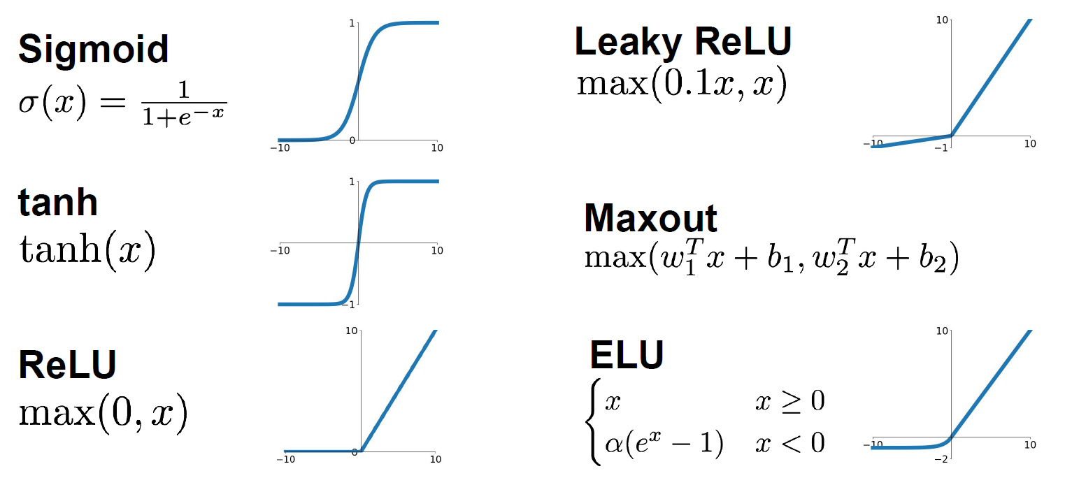
Activation Functions

Neural Networks, Architectures

1
2
3
4
5
6
# forward-pass of a 3-layer neural network:
f = lambda x: 1.0/(1.0 + np.exp(-x)) # activation function
x = np.random.randn(3,1) # random input vector of three numbers (3*1)
h1 = f(np.dot(W1, x) + b1) # calculate first hidden layer activations (4*1)
h2 = f(np.dot(W2, h1) + b2) # calculate second hidden layer activations (4*1)
out = np.dot(W3, h2) + b3 # output neuron (1*1)

5. Convolutional Neural Networks

We are going to learn about convolutional layers that reason on top of basically explicitly trying to maintain spatial structure.

A bit of history

Frank Rosenblatt ~1957: The Mark I Perceptron

Widrow and Hoff ~1960: Adaline/Madaline Start to stack the linear layers into multilayer perceptron networks

Rumelhart et al. ~1986: First time back-propagation become popular

LeCun, Bottou et al. ~1998: Gradient-based learning applied to document recognition

Hinton and Salakhutdinov ~2006: Reinvigorated research in Deep Learning

Krizhevsky, A., Sutskever, I. & Hinton, G.

ImageNet classification with deep convolutional neural networks.

This report was a breakthrough that used convolutional nets to almost halve the error rate for object recognition, and precipitated the rapid adoption of deep learning by the computer vision community.

Mohamed, A.-R., Dahl, G. E. & Hinton, G.

Acoustic modeling using deep belief networks.

Dahl, G. E., Yu, D., Deng, L. & Acero, A.

Context-dependent pre-trained deep neural networks for large vocabulary speech recognition.

Fast-forward to today: ConvNets are everywhere.

Convolution and pooling

Fully connected layer

Instead of stretching this all out into one long vector, we are now going to keep the structure of the image, the three dimensional input. We are going to convolve the filter with the image.

When we are dealing with a convolutional layer, we want to work with multiple filters. Because each filter is kind of looking for a specific type of template or concept in the input volume. Each of the filter is producing an activation map.

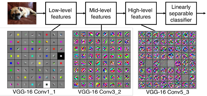
The filters at the earlier layers usually represent low-level features that you are looking for, such as edges etc. And you can get more complex kinds of features like corners and blobs at mid levels. In higher levels you are going to get things that are starting to more resemble concepts than blobs.

We call the layer convolutional because it is related to convolution of two signals:

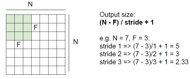
In practice, we are common to zero pad the border. In general, common to see Conv layers with stride 1, filters of size $F\times F$, and zero-padding with $(F-1)/2$. Without the padding, the input convolved with filters will shrink volumes spatially.

Example: Input volume: $32\times 32\times 3$, ten $5\times 5$ filters with stride 1 and pad 2. So what is the number of parameters in the layer?

$+1$ is for bias and $\times 3$ is for the depth.

Example: Conv layer in Torch and Caffe

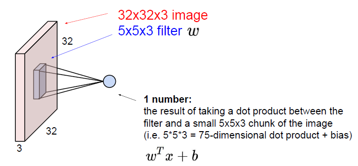
The brain view of Conv layer

The result of taking a dot product between the filter and the local part of the image is just like a neuron with local connectivity.

In the full connected layer, each neuron looks at the full input volume, compared to the Conv layer just looks at the local spatial region.

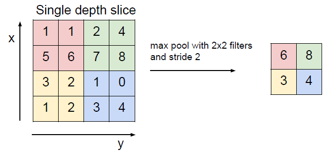
Polling layer

• Makes the representations smaller and more manageable
• Operates over each activation map independently

A common way to do this is max po0ling. The values can be considered as the activations of the neurons, so the max value is kind of how much this neuron fired in this location.

Conv Net demo (training on CIFAR-10)

6. Training Neural Networks: Part I

1. One time setup: activation functions, preprocessing, weight initialization, regularization, gradient checking
2. Training dynamics: babysitting the learning process, parameter updates, Hyperparameter optimization
3. Evaluation: model ensembles

Activation Functions

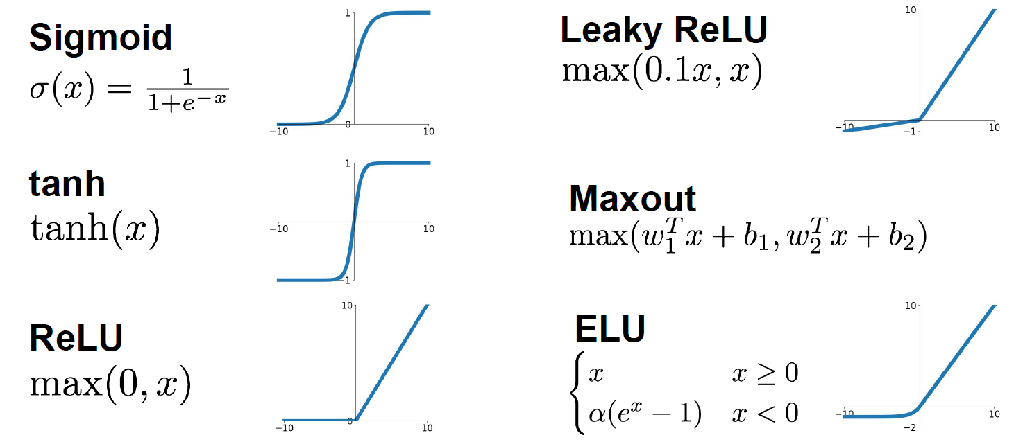
Sigmoid: $f(x) = 1/(1+e^{-x})$

It squashes numbers to range(0, 1). It is popular historically since it has nice interpretation as a saturating “firing rate” of a neuron.

Problems: The saturated neurons will kill the gradients when the absolute value of the input is too large. And the sigmoid outputs are not zero-centered. When the input $\vec{x}$ are all positive, it will lead to a zig zag path in the update process. This is also why we want zero-mean data. (More details are in the video.)

Tanh: $f(x) = tanh(x)$

It is zero centered, but it will still kill the gradients.

ReLU: $f(x) = \max(0,x)$

It does not saturate in the positive region and it converges much faster than the sigmoid and tanh. Actually, it also more biologically plausible than sigmoid.

Dead ReLU will never activate and never update.

In practice people also like to initialize ReLU with slightly positive biases, in order to increase the likelihood of it being active at initialization and to get some updates. And this basically just biases towards more ReLU firing at the beginning.

Leaky ReLU: $f(x) = max(0.01x,x)$

Parametric ReLU: $f(x)=max(\alpha x, x)$

Here is no saturates and it is computationally efficient. And it converges much faster than the sigmoid or tanh function in practice. In Parameter ReLU, the slope now is a parameter $\alpha$ that we can backprop into and learn, so this gives more flexibility.

Exponential Linear Units (ELU)

It has all benefits of ReLU and the negative saturation regime compared with Leaky ReLU adds some robustness to noise.

Max out: $f(x) = max(w_1^Tx+b_1, w_2^Tx+b_2)$

We use this function to generalizes ReLU and Leaky ReLU. It does not saturate so it does not die. But it doubles the number of parameters of neurons.

In practice:

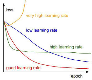
1. Use ReLU but be careful with your learning rates.
2. Try out Leaky ReLU or Max out or ELU.
3. Try out tanh but do not expect it much.
4. Do not use sigmoid.

Data Preprocessing

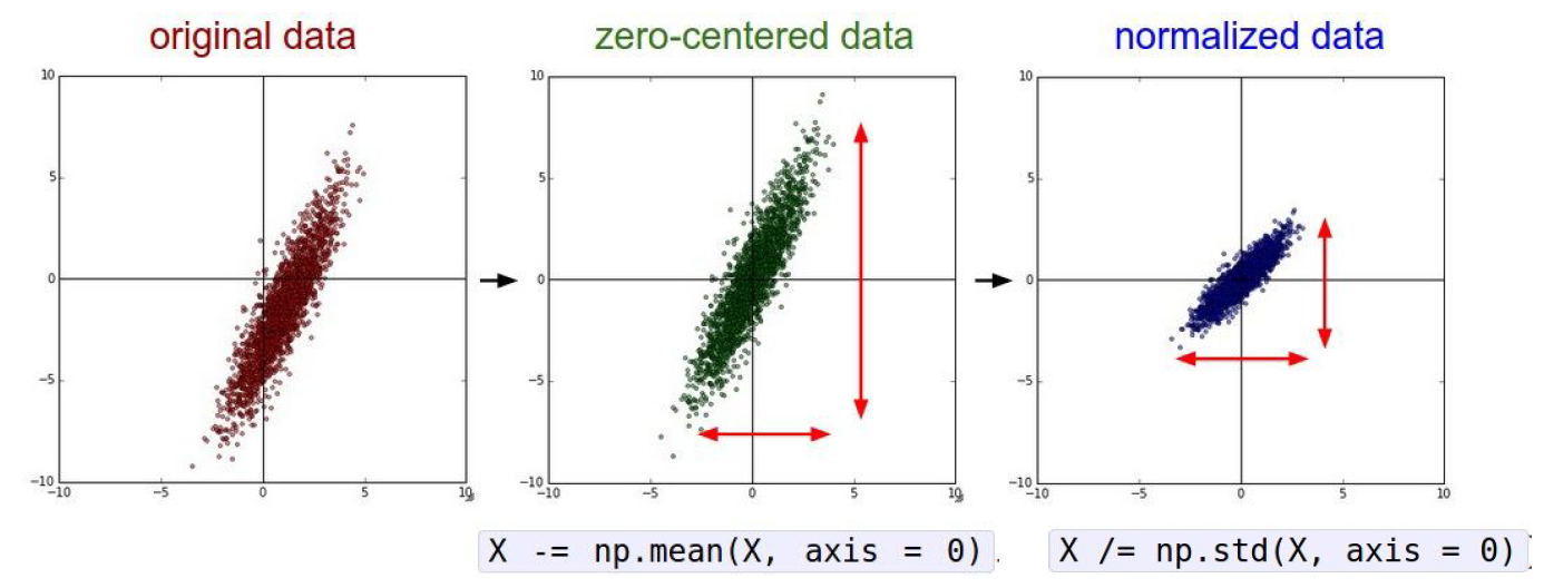
In practice, since for images, which is what we are dealing with here, for the most part, we will do the zero centering, but actually we do not normalize the pixels values because generally for images you can have relatively comparable scale and distribution at each location compared to more general machine learning problems.

For images, we always subtract the mean image or subtract per-channel mean. It is not common to normalize variance, such as doing PCA or whitening. Remember that the mean value is for the whole data set instead of one train batch.

Weight Initialization

If all the parameters are zero, all the neurons will do the same thing depending your input. They are going to update in the same way and you will get all neurons that they are exactly the same.

First idea: Small random numbers (Gaussian with zero mean and $10^{-2}$ standard deviation)

1
W = 0.01 * np.random.randn(D, H)

Works ok for small networks, but problems with deeper networks.

Xavier initialization: We specify that we want the variance of the input to be the same as a variance of the output, and then derive what the weight should be.

1
2
3
W = np.random.randn(fan_in, fan_out) / np.sqrt(fan_in)
# W = np.random.randn(fan_in, fan_out) / np.sqrt(fan_in / 2) for ReLU
# layer initialization

But when using the ReLU nonlinearity it breaks because it’s killing half of the units so it’s actually halving the variance that you get out of this.

Proper initialization is an active area of research

Batch Normalization

Keep activations in a Gaussian range that we want.

Actually, in stead of with weight initialization, we are setting this at the start of training, so that we try to get it into a good spot, which means we can get a unit Gaussian at every layer.

Compute the empirical mean and variance independently for each dimension. Usually inserted after fully connected or convolutional layers and before nonlinearity.

After the normalization, it allow the network to squash the range if it wants to. And the network can learn the parameters $\gamma$ and $\beta$ to recover the identity mapping.

• Improves the gradient flow through the network
• Allow higher learning rates and reduces the strong dependence on initialization
• Acts as a form of regularization in a funny way and slightly reduce the need for dropout.

Note that the mean and variance are not computed based on the batch. Instead, a single fixed empirical mean of activations during training is used. (E.g. It can be estimated during training with running averages)

Babysitting the Learning Process

1. Preprocess the data
2. Choose the architecture
3. Do some checks, which means to make sure that the loss function is reasonable and you can overfit very small portion of the training data.
4. Start from small regularization and find learning rate that makes the loss go down.

Hyperparameter Optimization

Network architecture, learning rate, decay schedule and update type, regularization

Cross validation strategy

Only a few epochs to get rough idea of what parameters work.

Note that it is best to optimize in log space, and using random search.

7. Training Neural Networks: Part II

Optimization

The kind of core strategy in training neural networks is an optimization problem. We write down some loss function and optimize the parameters of the network to minimize the loss function.

1
2
3
4
5
# Vanilla Gradient Descent
while True:
    weights_grad = evaluate_gradient(loss_fun, data, weights)
    # Parameters update
    weights += - step_size * weights_grad

But the stochastic gradient descent has some questions.

It is difficult to deal with the circumstances that loss change quickly in one direction but slowly in another. The SGD will has very slow progress along shallow dimension and jitter or zig-zag routes along the fast-changing dimensions. And it probably come much more common in high dimensions.

Another question is local minima or saddle point.

And SGD is stochastic gradient descent, and our gradients come from minibatches, so they can be noisy.

How about adding a momentum term to the stochastic gradient descent?

Actually adding momentum here can help us with this high condition number problem.

It can be thought as a smooth moving average of the recent gradients.

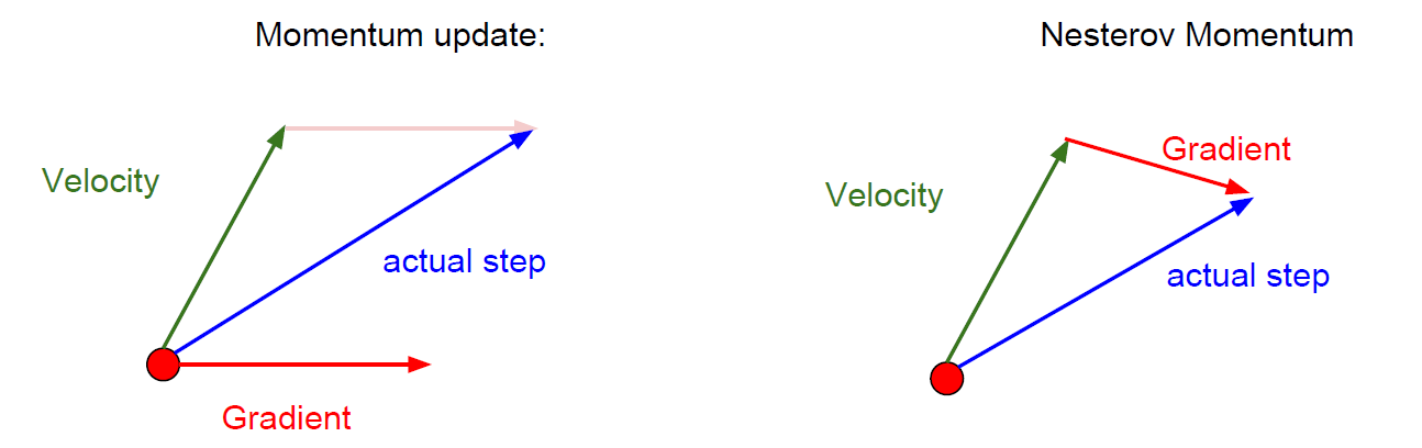
Nesterov Momentum

Change the variables and rearrange, we have:

AdaGrad

Added element-wise scaling of the gradient based on the historical sum of squares in each dimension.

1
2
3
4
5
grad_suqare = 0
while True:
    dx = compute_gradient(x)
    grad_squared += dx * dx
    x -= learning_rate * dx / (np.sqrt(grad_sqared) + 1e-7)

RMSProp

1
2
3
4
5
grad_suqare = 0
while True:
    dx = compute_gradient(x)
    grad_squared = decay_rate * grad_squared + (1 - decay_rate) * dx * dx
    x -= learning_rate * dx / (np.sqrt(grad_sqared) + 1e-7)

Adam

1
2
3
4
5
6
7
8
9
10
11
12
first_moment = 0
second_moment = 0
for t in range(num_iterations):
    dx = compute_gradient(x)
    # momentum
    first_moment = beta1 * first_moment + (1 - beta1) * dx
    second_moment = beta2 * second_moment + (1 - beta2) * dx * dx
    # bias corretion
    first_unbias = first_moment / (1 - beta1 ** t)
    second_ubias = second_moment / (1 - beta2 ** t)
    # AdaGrad or RMSProp
    x -= learning_rate * first_unbias / (np.sqrt(second_unbias) + 1e-7)

Bias correction for the fact that first and second moment estimates start at zero.

Adam with beta1 = 0.9, beta2 = 0.999, and learning_rate = 1e-3 or 5e-4 is a great starting point for many models!

Learning rate can decay over time, the methods including step decay, exponential decay or 1/t decay, etc.

First-order Optimization: Use gradient form linear approximation

Second-order Optimization: Use gradient and Hessian to form quadratic approximation.

second-order Taylor expansion

However, the matrix $H$ is $n\times n$, where $n$ is the network parameters, so this method is bad for deep learning. So we have Quasi-Newton methods (BGFS most popular): Instead of inverting the Hessian ($O(n^3)$), approximate inverse Hessian with rank 1 updates over time ($O(n^2)$ each).

L-BFGS usually works very well in full batch, deterministic mode. If you have a single, deterministic $f(x)$ then L-BFGS will probably work very nicely. But it does not transfer very well to mini-batch setting. Adapting L-BFGS to large-scale, stochastic setting is an active area of research.

Model Ensembles: Train multiple independent models and at test time average their results

Regularization: Dropout

In each forward pass, randomly set some neurons to zero. Probability of dropping is a hyper parameter; 0.5 is common. The dropout is usually added in full connected layers, but may also in convolution layers.

1
2
3
4
5
6
7
8
9
10
11
12
13
14
# probablility of keeping a unit sctive
p = 0.5
def train_step(X):
    # forward pass for example 3-layer neural network
    H1 = np.maximum(0, np.dot(W1, X) + b1)
    # first dropout mask
    U1 = np.random.rand(*H1.shape) < p
    H1 *= U1
    
    H2 = np.maximum(0, np.dot(W2, H1) + b2)
    # second dropout mask
    U2 = np.random.rand(*H2.shape) < p
    H2 *= U2
    out = np.dot(W3, H2) + b3

An interpretation is dropout is training a large ensemble of models that share parameters. For example, an FC layer with 4096 units has $2^{4096}$~ $10^{1233}$ possible masks!

Dropout makes our output random, so we want to average out the randomness at test time using the formula:

At test time, we just multiply by dropout probability, and now the expected values are the same.

1
2
3
4
5
def predict(X):
    # scale the activations
    H1 = np.maximum(0, np.dot(W1, X) + b1) * p
    H2 = np.maximum(0, np.dot(W2, H1) + b2) * p
    out = np.dot(W3, H2) + b3

Regularization: A common pattern

When we are training, we can add some kind of randomness. And we average out randomness (sometimes approximate) at testing time.

Regularization: Data Augmentation

We can randomly transform the image in some way during training such that the label is preserved. And we train on these random transformations of the image rather than the original images.

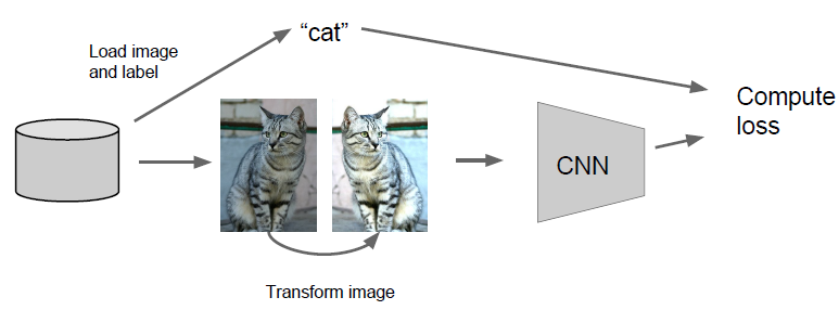
Translation, rotation, stretching, shearing, lens distortions…

Regularization Examples: Dropout, Batch Normalization, Data Augmentation, Drop Connect, Fractional Max Pooling, Stochastic Depth…

Transfer Learning

You can download big networks that were pre-trained on some dataset and then tune them for your own problem. And this is on way that you can attack a lot of problems in deep learning, even if you don’t have a big dataset of your own.

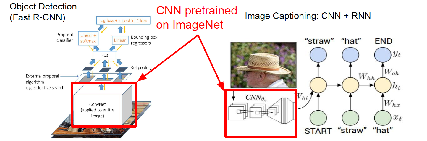
Deep learning frameworks provide a “Model Zoo” of pre-trained models so you don’t need to train your own.

8. Deep Learning Software

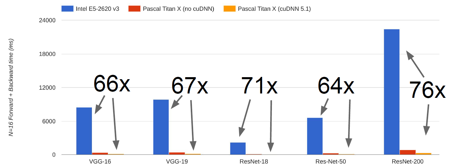
CPU vs GPU

GPU: Graphics Processing Unit. More cores, but each core is much slower and “dumber”; great for parallel tasks.

CPU: Fewer cores, but each core is much faster and much more capable; great at sequential tasks.

If you aren’t careful, training can bottleneck on reading data and transferring to GPU! Solutions:

• Read all data into RAM
• Use SSD instead of HDD
• Use multiple CPU threads to prefetch data

Deep Learning Framework

The point of deep learning frameworks:

1. Easily build big computational graphs.
2. Easily compute gradients in computational graphs.
3. Run it all efficiently on GPU (wrap cuDNN, cuBLAS, etc)

Here is an example of Computational Graphs.

In numpy:

1
2
3
4
5
6
7
8
9
10
11
12
13
14
15
16
17
18
import numpy as np
np.random.seed(0)

N, D = 3, 4
x = np.random.randn(N, D)
y = np.random.randn(N, D)
z = np.random.randn(N, D)

a = x * y
b = a + z
c = np.sum(b)

grad_c = 1.0
grad_b = grad_c * np.ones((N, D))
grad_a = grad_b.copy()
grad_z = grad_b.copy()
grad_x = grad_a * y
grad_y = grad_a * x

In TensorFlow:

1
2
3
4
5
6
7
8
9
10
11
12
13
14
15
16
17
18
19
20
21
22
23
24
25
import numpy as np
import tensorflow as tf
np.random.seed(0)

N, D = 3, 4

with tf.device('/gpu:0'):
    x = tf.placeholder(tf.float32)
    y = tf.placeholder(tf.float32)
    z = tf.placeholder(tf.float32)
    
    a = x * y
    b = a + z
    c = tf.reduce_sum(b)
    
grad_x, grad_y, grad_z = tf.gradients(c, [x, y, z])

with tf.Session() as sess:
    values = {
        x: np.random.randn(N, D),
        y: np.random.randn(N, D),
        z: np.random.randn(N, D)
    }
    out = sess.run([c, grad_x, grad_y, grad_z], feed_dict=values)
    c_val, grad_x_val, grad_y_val, grad_z_val = out

In Pytorch:

1
2
3
4
5
6
7
8
9
10
11
12
13
14
15
16
17
import numpy as np
import torch
from torch.autograd import Variable

N, D = 3, 4

x = Variable(torch.randn(N, D).cuda(), requires_grad = True)
y = Variable(torch.randn(N, D).cuda(), requires_grad = True)
z = Variable(torch.randn(N, D).cuda(), requires_grad = True)

a = x * y
b = a + z
c = torch.sum(b)

c.backward()

print(x.grad.data, y.grad.data, z.grad.data)

TensorFlow

Running example: Train a two-layer ReLU network on random data with L2 loss

1
2
3
4
5
6
7
8
9
10
11
12
13
14
15
16
17
18
19
20
21
22
23
24
25
26
27
28
29
30
31
32
33
import numpy as np
import tensorfloww as tf

# Define the computional graph
N, D, H = 64, 1000, 100
# Create placeholders for input x, weights w1 and w2, and targets y
x = tf.placeholder(tf.float32, shape=(N, D))
y = tf.placeholder(tf.float32, shape=(N, D))
w1 = tf.placeholder(tf.float32, shape=(D, H))
w2 = tf.placeholder(tf.float32, shape=(H, D))

# Forward pass
# No computation happens here - just building the graph!
h = tf.maximum(tf.matmul(x, w1), 0)
y_pred = tf.matmul(h, w2)
diff = y_pred -y
loss = tf.reduce_mean(tf.reduce_sum(diff ** 2, axis=1))
# Tell TensorFlow to compute loss of gradient with respect to w1 and w2.
grad_w1, grad_w2 = tf.gradients(loss, [w1, w2]) 

# We enter a session so we can actually run the graph
with tf.Session() as sess:
    # Create numpy arrays that will fill in the placeholders above
    values = {
        x: np.random.randn(N, D),
        y: np.random.randn(N, D),
        w1: np.random.randn(H, D),
        w2: np.random.randn(N, D)
    }
    
    # Run the graph
    out = sess.run([loss, grad_w1, grad_w2], feed_dict=values)
    loss_val, grad_w1_val, grad_w2_val = out

Using high level API:

1
2
3
4
5
6
7
8
9
10
11
12
13
14
15
16
17
18
19
20
21
22
23
N, D, H = 64, 1000, 100
x = tf.placeholder(tf.float32, shape=(N, D))
y = tf.placeholder(tf.float32, shape=(N, D))

# Use Xavier initializer
init = tf.contrib.layers.xavier_initializier()
# Setup weight and bias automatically
h = tf.layers.dense(inputs=x, units=H, activation=tf.nn.relu, kernel_initializer=init)
y_pred = tf.layers.dense(inputs=h, units=D, kernel_initializer=init)

# Use predefined common losses
loss = tf.losses.mean_squared_error(y_pred, y)

# Use an optimizer to compute gradients and update weights
optimizer = tf.train.GradientDescentOptimizer(1e0)
updates = optimizer.minimize(loss)

with tf.Session() as sess:
    sess.run(tf.global_variables_initializer())
    values = {x: np.random.randn(N, D),
              y: np.random.randn(N, D),}
    for t in range(50):
        loss_val, _ = sess.run([loss, updates], feed_dict=values)

Keras: Keras is a layer on top of TensorFlow, makes common things easy to do.

Other high level wrappers:

• Keras
• TFLearn
• TensorLayer
• tf.layers
• TF-Slim
• tf.contrib.learn
• Pretty Tensor
• Sonnet

Pytorch

Three level of abstraction:

1. Tensor: Imperative ndarray, but runs on GPU.
2. Variable: Node in a computational graph; stores data and gradient.
3. Module: A neural network layer; may store state or learn-able weights.

A Pytorch Variable is a node in a computational graph.

1. x.data is a Tensor
2. x.grad is a Variable of gradients (same shape as x.data)
3. x.grad.data is a Tensor of gradients

1
2
3
4
5
6
7
8
9
10
11
12
13
14
15
16
17
18
19
20
21
22
23
24
25
import torch
from torch.autograd import Variable

N, D_in, H, D_out = 64, 1000, 100, 10
# PyTorch Tensors and Variables have the same API!
# Variables remember how they were created (for backprop)
x = Variable(torch.randn(N, D_in), requires_grad=False)
y = Variable(torch.randn(N, D_out), requires_grad=False)

# We want gradients with respect to weights instead of data
w1 = Variable(torch.randn(D_in, H), requires_grad=True)
w2 = Variable(torch.randn(H, D_out), requires_grad=True)

learning_rate = 1e-6
for t in range(500):
    y_pred = x.mm(w1).clamp(min=0).mm(w2)
    loss = (y_pred - y).pow(2).sum()
    
    if w1.grad: w1.grad.data.zero_()
    if w2.grad: w2.grad.data.zero_()
    loss.backward()
    
    # Make gradient step on weights
    w1.data -= learning_rate * w1.grad.data
    w2.data -= learning_rate * w2.grad.data

In TensorFlow, we building up the explicit graph, then running the graph many times. But in Pytorch, instead we are building up a new graph every time we do a forward pass.

In Pytorch, you can Define your own autograd functions by writing forward and backward for Tensors. Then you can use our new autograd function in the forward pass.

Using high level API: Pytorch:nn

1
2
3
4
5
6
7
8
9
10
11
12
13
14
15
16
17
18
19
20
21
22
23
24
25
26
27
import torch
from torch.autograd import Variable

N, D_in, H, D_out = 64, 1000, 100, 10
x = Variable(torch.randn(N, D_in))
y = Variable(torch.randn(N, D_out), requires_grad=False)

# Defined the model as a sequence of layers
# nn also defines common loss function
model = torch.nn.Sequential(
    torch.nn.Linear(D_in, H),
    torch.nn.ReLU(),
    torch.nn.Linear(H, D_out))
loss_fn = torch.nn.MSELoss(size_average=False)
# Define the optimization function
learning_rate = 1e-4
optimizer = torch.optim.Adam(model.parameters(), lr=learning_rate)

for t in range(500):
    # Forward pass: feed data to model and calculate the loss function
    y_pred = model(x)
    loss = loss_fn(y_pred, y)
    # Backward pass to calculate all gradients
    optimizer.zero_grad()
    loss.backward()
    
    optimizer.step()

A DataLoader wraps a Dataset and provides minibatching, shuffling, multithreading, for you. When you need to load custom data, you can just write your own Dataset class

Static graphs and Dynamic graphs

• TensorFlow: Build graph once, then run many times (static)
• Pytorch: Each forward pass defines a new graph (dynamic)

• Previous
  Essense of Linear Algebra
• Next
  Deep Learning for Computer Vision II