Here is the second half part of the notes for CS231n: Convolutional Neural Networks for Visual Recognition from Stanford University. This part includes the different network architectures, some applications and advanced topics.
9. CNN Architectures
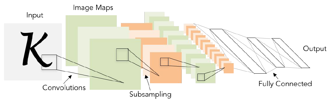
LeNet-5 [LeCun et al., 1998]
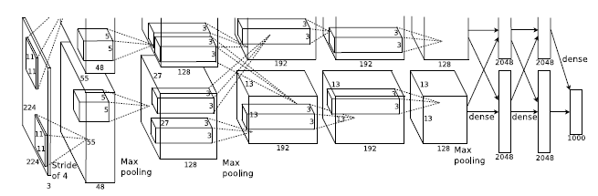
AlexNet [Krizhevsky et al., 2012]
CONV1, MAX POOL1. NORM1, CONV2, MAX POOL2, NORM2,
CONV3, CONV4, CONV5, Max POOL3, FC6, FC7, FC8
Input: $227\times 227\times 3$ images
- First layer (CONV1): $96\ 11\times11$ filters applied at stride 4, so the output volume is $55\times 55\times 96$.
- Second layer (POOL1): 3x3 filters applied at stride 2, so the output volume is $27\times 27\times 96$.
Historical note: Trained on GTX 580GPU with only 3 GB of memory. Network spread across 2 GPUs, half the neurons (feature maps) on each GPU.
ZFNet [Zeiler and Fergus, 2013]
Some updates of hyperparameters in AlexNet.
VGGNet [Simonyan and Zisserman, 2014]
It has small filters (only $3\times 3$ conv filters) and deeper networks.
Stack of three $3\times3$ conv (stride 1) layers has same effective receptive field as one $7\times7$ conv layer. So with small filters, you can get a deeper architecture with more non-linearities and fewer parameters.
It has most memory in early convolutional layers and late fully connect layers.
- Total memory: approximately 96MB per image
- Total parameters: 138M parameters.
- FC7 features can generalize well to other tasks.
Network in Network [Lin et al., 2014]
MLP conv layer with “micro-network” within each conv layer to compute more abstract features for local patches.
Precursor to GoogLeNet and ResNet “bottleneck” layers.
GoogLeNet [Szegedy et al., 2014]
It focus on thee problem of computational efficiency and it try to design a network architecture that was very efficient in the amount of compute. It used the inception module and no fully connect layers.
It only have 5 million parameters which is 12 times less than AlexNet.
“Inception module”: design a good local network topology (network within a network) and then stack these modules on top of each other. It apply parallel filter operations on the input from previous layer such as multiple receptive field sizes for convolution ($1\times1, 3\times3, 5\times5$) or pooling operation ($3\times3$), and then concatenate all filter outputs together depth-wise.
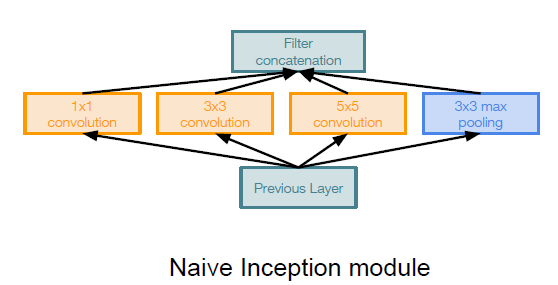
Problem: computational complexity. Pooling layer also preserves feature depth, which means total depth after concatenation can only grow at every layer!
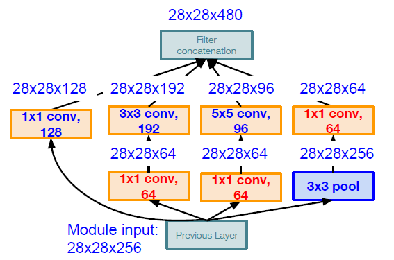
Solution: using $1\times 1$ convolutional layers to deduce the feature depth
It has auxiliary classification outputs to inject additional gradient at lower layers.
ResNet [He et al., 2015]
When we continue stacking deeper layers on a “plain” convolutional neural network, it performs worse.
There is a hypothesis that the problem is an optimization problem and deeper models are harder to optimize because the deeper model should be able to perform at least as well as the shallower model.
Solution: Use network layers to fit a residual mapping instead of directly trying to fit a desired underlying mapping.
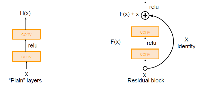
Use layers to fit residual $F(x) = H(x) - x$ instead of $H(x)$ directly.
When upstream gradient is coming in through an addition gate, then it will split and fork along two different paths. So it will take one path through the convolutional blocks, but it will also have a direct connection of the gradient through the residual connection. The residual connection can give a sort of gradient super highway for gradient to flow backward through the entire network. And this allow it to train much easier and much faster.
Full ResNet architecture
- Stack residual blocks
- Every residual block has two 3x3 conv layers.
- Total depths of 34, 50, 101, or 152 layers for ImageNet
For deeper networks (ResNet-50+), use “bottleneck” layer to improve efficiency (similar to GoogLeNet).
Other nets
-
Identity Mappings in Deep Residual Networks [He et al., 2016]
-
Wide Residual Networks [Zagoruyko et al., 2016]
-
ResNeXt [Xie et al., 2016]
-
Deep Networks with Stochastic Depth [Huang et al. 2016]
-
FractalNet [Larsson et al. 2017]
-
Densely Connected Convolutional Networks [Huang et al. 2017]
-
SqueezeNet [Iandola et al. 2017]
10. Recurrent Neural Networks
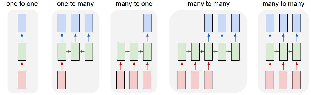
Vanilla Neural Networks: We receive some input which is a fixed size object. That input is fed through some set of hidden layers and produces a single output like a set of classification scores over a set of categories.
Recurrent Neural Networks: Process Sequences
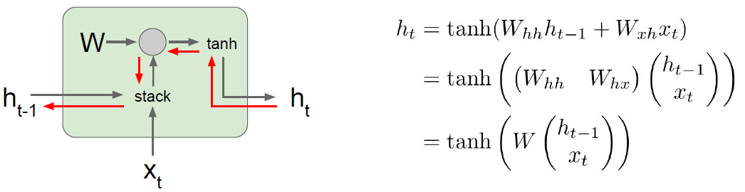
Recurrent neural network has its little recurrent core cell, and it will take some input x and feed that into the RNN. RNN has some internal hidden state, which may be updated every time that the RNN reads a new input. The internal hidden state will be feed back to the model the next time it reads an input.
We can process a sequence of vectors x by applying a recurrence formula at every time step. And the same function and the same set of parameters are used at every time step.
\[h_t = f_W(h_{t-1}, x_t)\]RNN: Computational Graph: Many to Many
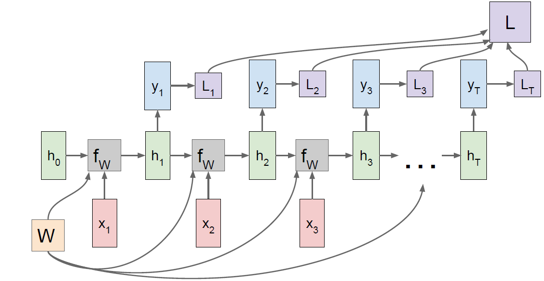
We are reusing the W matrix at every time step of the computation. You will have a separate gradient for W flowing from from each of the time steps, and then the final gradient for W will be the sum of all of these individual per time step gradients.
Sequence to Sequence: Many-to-one + one-to-many
- Many to one: Encode input sequence in a single vector
- One to many: Produce output sequence from single input vector
Example: Character-level Language Model Sampling
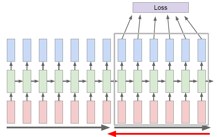
Truncated Backpropagation through time
Run forward and backward through chunks of the sequence instead of whole sequence. Carry hidden states forward in time forever, but only backpropagate for some smaller number of steps.
Karpathy, Johnson, and Fei-Fei: Visualizing and Understanding Recurrent Networks, ICLR Workshop 2016
Image captioning
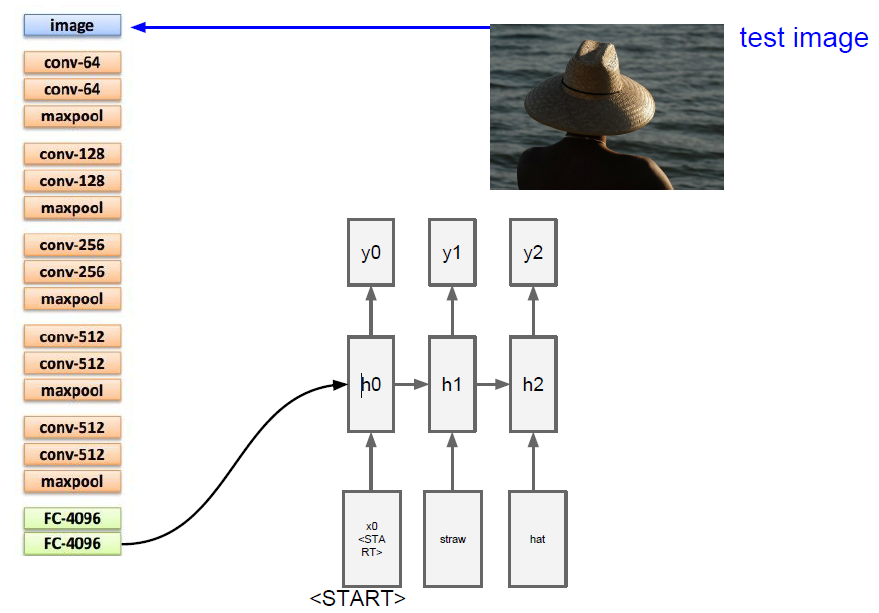
This model work pretty well when you ask them to caption images that were similar to the training data, but they definitely have a hard time generalizing far beyond that.
Image Captioning with Attention
RNN focuses its attention at a different spatial location when generating each word.
The convolutional network rather than producing a single vector summarizing the entire image, now it produce some grid of vectors that give maybe one vector for each spatial location in the image.
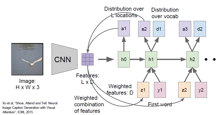
The module will have two outputs, one is the distribution over vocabulary words, the other is the distribution over image locations. This whole process will continue and it will sort of do these two different things at every time step.
Hard attention vs Soft attention
Visual Question Answering
Multilayer RNNs
Vanilla RNN Gradient Flow
Backpropagation from $h_t$ to $h_{t-1}$ multiplies by $W_{hh}^T$. So computing gradient of $h_0$ involves many factors of $W$. So when the largest singular value < 1, it called vanishing gradients; when the largest singular value > 1, it called exploding gradients.
The method to deal with exploding gradients problem is called gradient clipping, which means scale computing gradient gradient if its norm is too big. And the vanishing gradients problems inspire the development of LSTM.
Long Short Term Memory (LSTM)
A common variant on the vanilla RNN is the Long-Short Term Memory (LSTM) RNN. Vanilla RNNs can be tough to train on long sequences due to vanishing and exploding gradients caused by repeated matrix multiplication. LSTMs solve this problem by replacing the simple update rule of the vanilla RNN with a gating mechanism as follows.
Similar to the vanilla RNN, at each timestep we receive an input $x_t\in\mathbb{R}^D$ and the previous hidden state $h_{t-1}\in\mathbb{R}^H$; the LSTM also maintains an $H$-dimensional cell state, so we also receive the previous cell state $c_{t-1}\in\mathbb{R}^H$. The learnable parameters of the LSTM are an input-to-hidden matrix $W_x\in\mathbb{R}^{4H\times D}$, a hidden-to-hidden matrix $W_h\in\mathbb{R}^{4H\times H}$ and a bias vector $b\in\mathbb{R}^{4H}$.
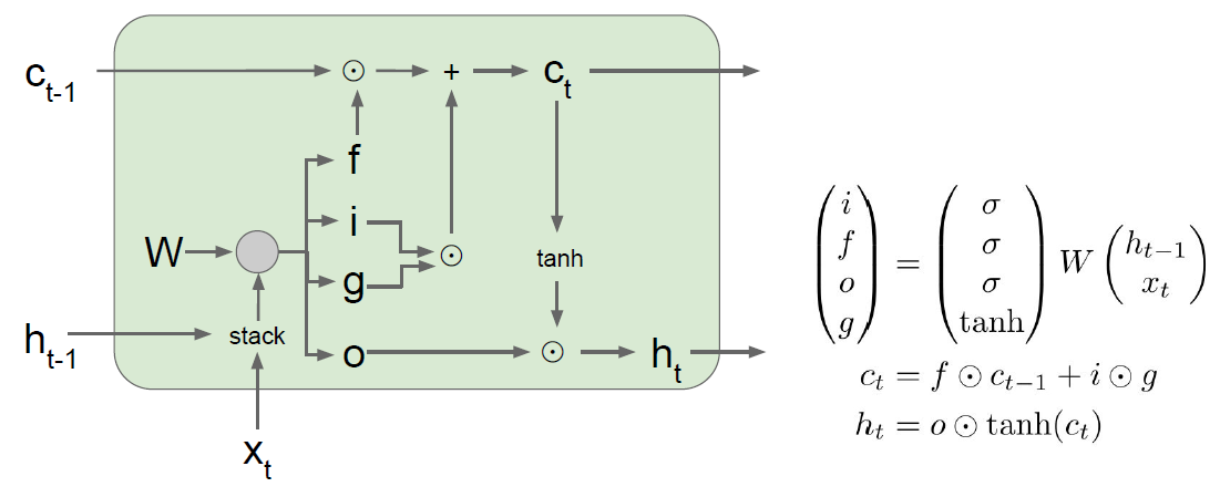
At each timestep we first compute an activation vector $a\in\mathbb{R}^{4H}$ as $a=W_xx_t + W_hh_{t-1}+b$. We then divide this into four vectors $a_i,a_f,a_o,a_g\in\mathbb{R}^H$ where $a_i$ consists of the first $H$ elements of $a$, $a_f$ is the next $H$ elements of $a$, etc. We then compute the input gate $g\in\mathbb{R}^H$, forget gate $f\in\mathbb{R}^H$, output gate $o\in\mathbb{R}^H$ and block input $g\in\mathbb{R}^H$ as
\[i = \sigma(a_i) \hspace{2pc} f = \sigma(a_f) \hspace{2pc} o = \sigma(a_o) \hspace{2pc} g = \tanh(a_g)\]where $\sigma$ is the sigmoid function and $\tanh$ is the hyperbolic tangent, both applied elementwise.
Finally we compute the next cell state $c_t$ and next hidden state $h_t$ as
\[c_{t} = f\odot c_{t-1} + i\odot g \hspace{4pc} h_t = o\odot\tanh(c_t)\]where $\odot$ is the elementwise product of vectors.
In the rest of the notebook we will implement the LSTM update rule and apply it to the image captioning task.
In the code, we assume that data is stored in batches so that $X_t \in \mathbb{R}^{N\times D}$ and will work with transposed versions of the parameters: $W_x \in \mathbb{R}^{D \times 4H}$, $W_h \in \mathbb{R}^{H\times 4H}$ so that activations $A \in \mathbb{R}^{N\times 4H}$ can be computed efficiently as $A = X_t W_x + H_{t-1} W_h$
Backpropagation from $c_t$ to $c_{t-1}$ only elementwise multiplication by $f$, no matrix multiply by $W$. So it has an uninterrupted gradient flow similar to ResNet , which can control the vanishing gradient.
Other RNN Variants
- GRU [Cho et al. 2014]
- An Empirical Exploration of Recurrent Network Architectures [Jozefowicz et al., 2015]
11. Detection and Segmentation
From image classification to detection, localization and segmentation
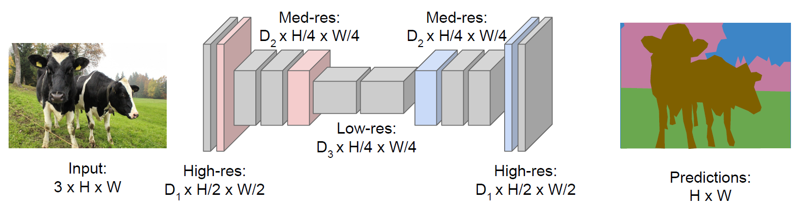
Segmentation
We want to produce a category label for each pixel of the input image, and this is called semantic segmentation. It don’t differentiate instance, and only care about pixels.
Sliding window: we take a input image and we break it up into many small, tiny local crops of the image. We can take each of this crops and treat this as a classification problem, saying for this crop, what is the category of the central pixel of the crop. And then we can use all the same machinery that we have developed for classifying entire images.
Problem: Very inefficient and super highly computational expensive.
Fully Convolutional: Design a network as a bunch of convolutional layers to make predictions for pixels all at once!
Problem: Convolutions at original image resolution will also be very expensive. So we can design network as a bunch of convolutional layers, with downsampling and upsampling inside the network!
Upsampling
-
Unpooling: nearest neighbor or “Bed of Nails”
- Max Unpooling: Corresponding pairs of downsampling and upsampling layers, then remember which element was max so that we can use that positions from pooling layers.
- Transpose Convolution or deconvolution, upconvolution
Classification and localization
We have two fully connected layers, for the first one we calculate the class score, and for the next one, we can get the box coordinates by treating the localization as a regression problem.
multi-task loss: using some hyperparameters to change the weight of two different loss
Human pose estimation: output some fixed number of coordinates of each joints
Object detection
Different from localization because there might be differing numbers of objects for each image, so the regression outputs are different.
Sliding window: Apply a CNN to many different crops of the image, CNN classifies each crop as object or background.
Problem: Need to apply CNN to huge number of locations and scales, very computationally expensive!
Region proposals: Find “blobby” image regions that are likely to contain objects, which just like traditional image processing methods. And it can run relatively fast. e. g. Selective Search gives 1000 region proposals in a few seconds on CPU.
Region based method
R-CNN
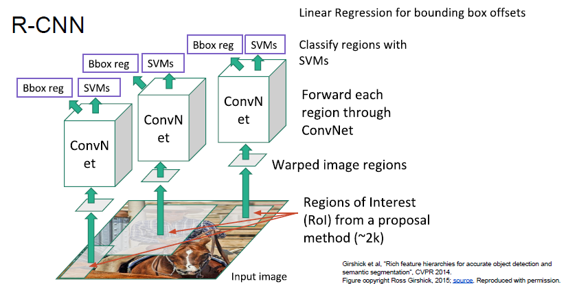
The R-CNN has ad hoc training objectives and the training and inference are slow and takes a lot of disk space.
Fast R-CNN
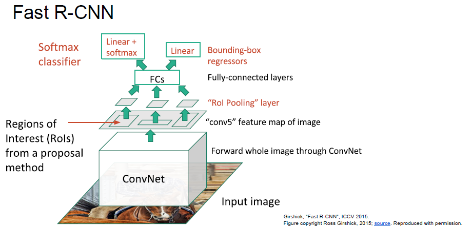
Problem: Runtime dominated by computing region proposals!
Faster R-CNN
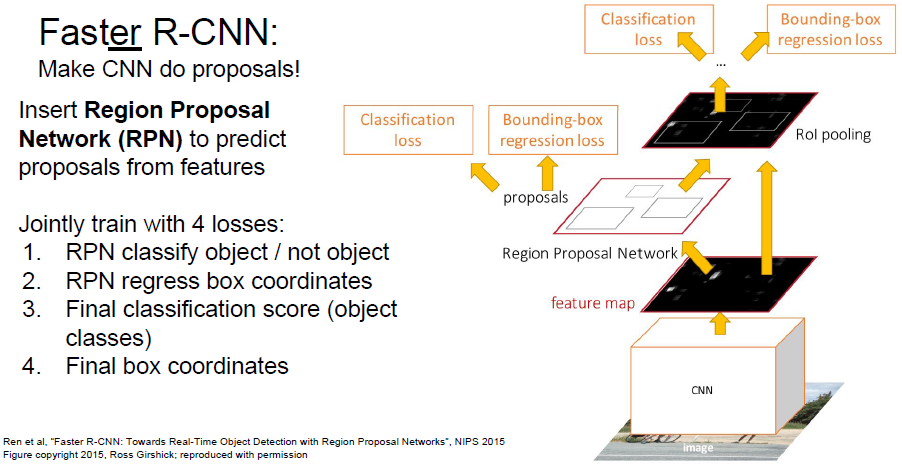
Detection without proposals
Yolo/SSD: Rather that doing independent processing for each of these potential regions, instead we want to try to treat this like a regression problem and just make all these predictions all at once with some big convolutional network.
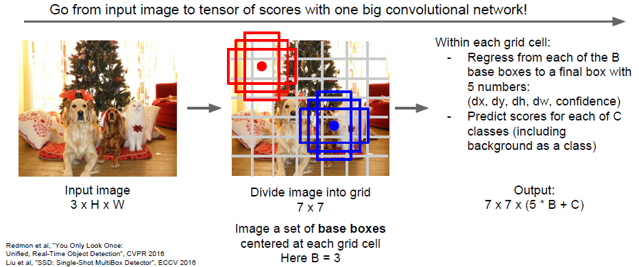
So we can see the object detection as this input of an image and output of a three dimensional tensor, and you can train the whole things with a giant convolutional network.
Instance Segmentation
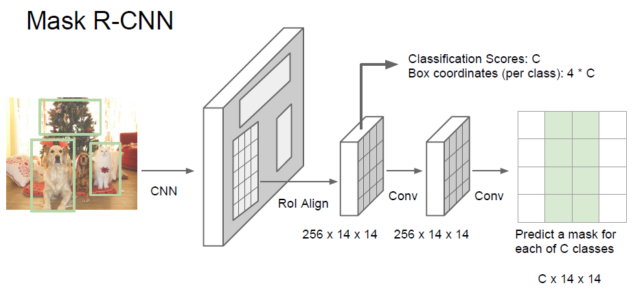
It has very good results, and it can also do pose estimation.
12. Visualizing and Understanding
What is going on inside convolutional networks?
First Layer: Visualize Filters
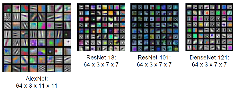
You can see a lot of things looking for oriented edges, likes bars of light and dark in various angles and various positions. We also can see opposing colors like green and pink or orange and blue. These convolutional networks seem to do something similar as human visual systems at their first layer.
If we draw this exact same visualization for the intermediate convolutional layers, it is actually a lot less interpretable.
Last Layer: Nearest Neighbors
We can record the 4096 dimensional vectors of a small batch of images in the last layer and using nearest neighbors approach in feature space.
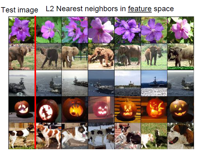
The pixels are often quite different between the image in it’s nearest neighbors and feature space. However, the semantic content of those images tends to be similar in this feature space, which means their features in the last layer are capturing some of those semantic content of these images.
Dimensionality Reduction
Visualize the “space” of feature vectors by reducing dimensionality of vectors from 4096 to 2 dimensions.
Simple algorithm: Principle Component Analysis (PCA) More complex: t-SNE
Reference: http://cs.stanford.edu/people/karpathy/cnnembed/
Visualizing Activations
Yosinski et al, “Understanding Neural Networks Through Deep Visualization”, ICML DL Workshop 2014.
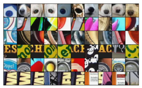
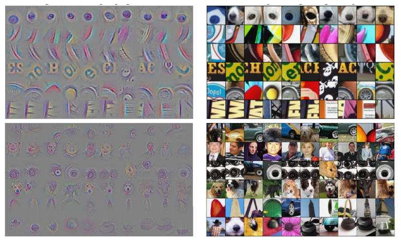
Maximally Activating Patches
Pick a layer and a channel (e.g. conv5 is 128 x 13 x 13, pick channel 17/128) Run many images through the network, record values of chosen channel and visualize image patches that correspond to maximal activations.
Springenberg et al, “Striving for Simplicity: The All Convolutional Net”, ICLR Workshop 2015
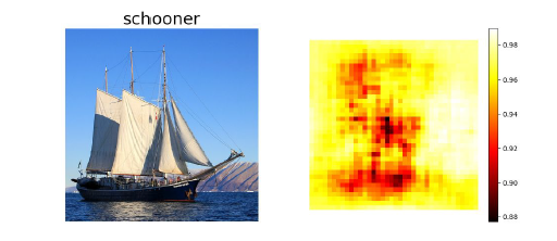
Occlusion Experiments
Mask part of the image before feeding to CNN, draw heatmap of probability at each mask location.
Zeiler and Fergus, “Visualizing and Understanding Convolutional Networks”, ECCV 2014
Saliency Maps
Simonyan, Vedaldi, and Zisserman, “Deep Inside Convolutional Networks: Visualizing Image Classification Models and Saliency Maps”, ICLR Workshop 2014.
Compute gradient of (unnormalized) class score with respect to image pixels, take absolute value and max over RGB channels. This will directly tell us in this sort of first order approximation sense. For each pixels in this input image, if we wiggle this pixel a little bit, then how much the classification score for the class change.
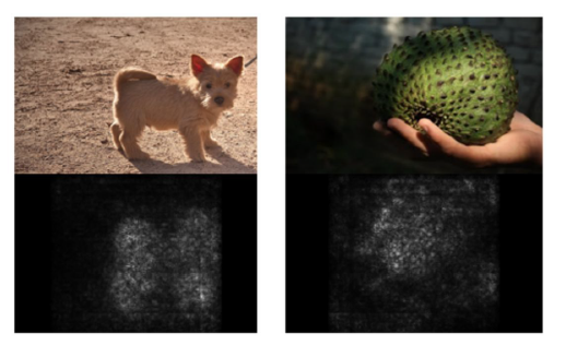
When you combine the Saliency Map with a segmentation algorithm called Grabcut, then you can, in fact, sometimes segment out the object in the image.
Guided backpropagation
Compute gradient of neuron value with respect to image pixels.
Images come out nicer if you only backprop positive gradients through each ReLU (guided backprop).
Zeiler and Fergus, “Visualizing and Understanding Convolutional Networks”, ECCV 2014
Springenberg et al, “Striving for Simplicity: The All Convolutional Net”, ICLR Workshop 2015
Gradient Ascent
Generate a synthetic image that maximally activates a neuron. \(I^* = \arg\max_If(I) + R(I)\)
- Initialize image to zeros
- Forward image to compute current scores (score of class before softmax)
- Backprop to get gradient of neuron value with respect to image pixels
- Make a small update to the image
regularizing: Penalize L2 norm of generated image, Gaussian blur image, Clip pixels with small values or gradients to 0
Use the same approach to visualize intermediate features
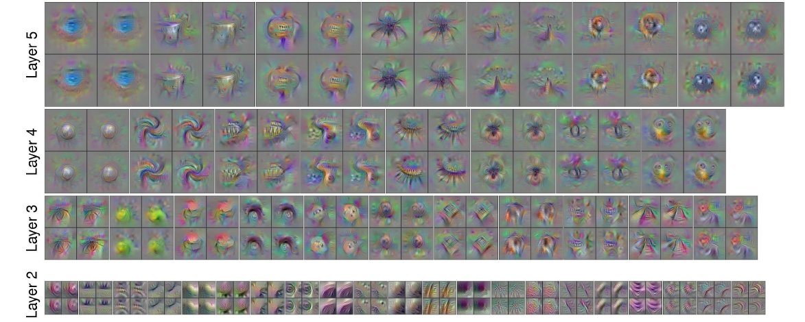
Adding “multi-faceted” visualization gives even nicer results. (Plus more careful regularization, center-bias)
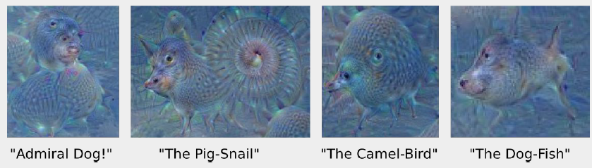
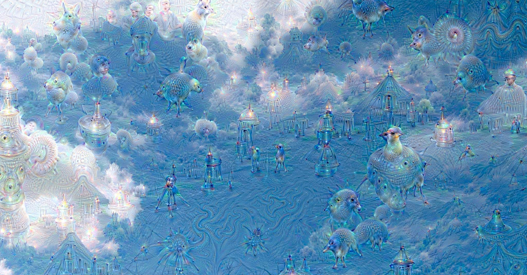
Deep Dream
Rather than synthesizing an image to maximize a specific neuron, instead try to amplify the neuron activations at some layer in the network.
- Forward: compute activations at chosen layer
- Set gradient of chosen layer equal to its activation, which is equivalent to $I^*=\arg\max_I\sum_if_i(I)^2$
- Backward: Compute gradient on image
- Update image
Feature Inversion
Given a CNN feature vector for an image, find a new image that:
- Matches the given feature vector
- “looks natural” (image prior regularization)
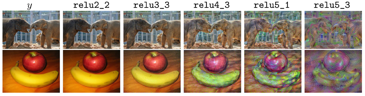
Function $l$ is used to measure the distance between the feature of the new image and the given feature vector. And the total variation regularizing function is used to encourage the spatial smoothness.
Mahendran and Vedaldi, “Understanding Deep Image Representations by Inverting Them”, CVPR 2015
Texture Synthesis
Nearest Neighbor
Using Gram Matrix
Each layer of CNN gives $C \times H \times W$ tensor of features: $H\times W$ grid of $C$ dimensional vectors. Outer product of two C-dimensional vectors gives $C \times C$ matrix measuring co-occurrence. Average over all $H W$ pairs of vectors, giving Gram matrix of shape $C \times C$.
- Pretrain a CNN on ImageNet (VGG-19)
- Run input texture forward through CNN, record activations on every layer; layer i gives feature map of shape $C_i \times H_i \times W_i$
- At each layer compute the Gram matrix giving outer product of features:
- Initialize generated image from random noise.
- Pass generated image through CNN, compute Gram matrix on each layer.
- Compute loss: weighted sum of L2 distance between Gram matrices. Backprop to get gradient on image.
- Make gradient step on image and do the same process.
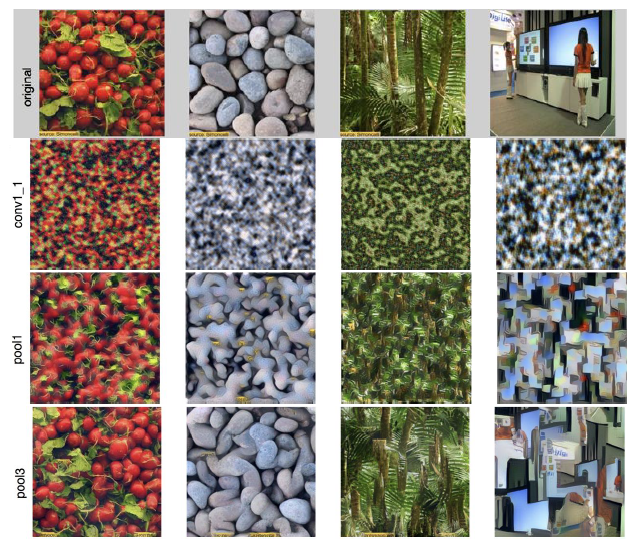
Reconstructing texture from higher layers recovers larger features from the input texture.
Neural Style Transfer
Feature + Gram Reconstruction
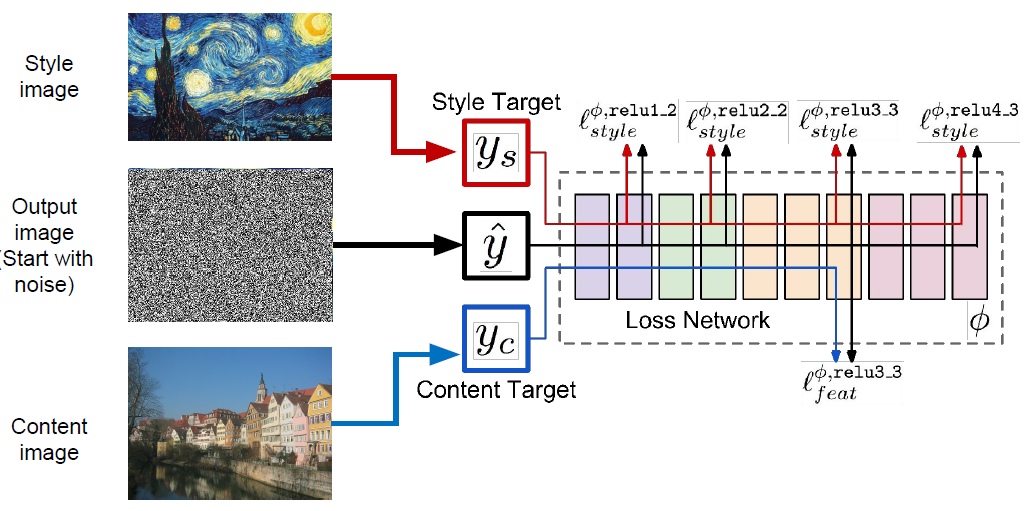
Gatys, Ecker, and Bethge, “Image style transfer using convolutional neural networks”, CVPR 2016
Fast Style Transfer
- Train a feed-forward network for each style
- Use pretrained CNN to compute same losses as before
- After training, stylize images using a single forward pass
Johnson, Alahi, and Fei Fei” Perceptual Losses for Real-Time Style Transfer and Super-Resolution”, ECCV 2016
One Network, Many Styles
Use the same network for multiple styles using conditional instance normalization: learn separate scale and shift parameters per style
Dumoulin, Shlens, and Kudlur, “A Learned Representation for Artistic Style”, ICLR 2017.
13. Generative Models
Supervised vs Unsupervised Learning
Supervised Learning: Data: (x, y), x is data, y is label Goal: Learn a function to map x -> y Examples: Classification, regression, object detection, semantic segmentation, image captioning, etc.
Unsupervised Learning: Data: x, Just data, no labels! Goal: Learn some underlying, hidden structure of the data Examples: Clustering, dimensionality reduction, feature learning, density estimation, etc.
Generative Models
Given training data, generate new samples from same distribution.
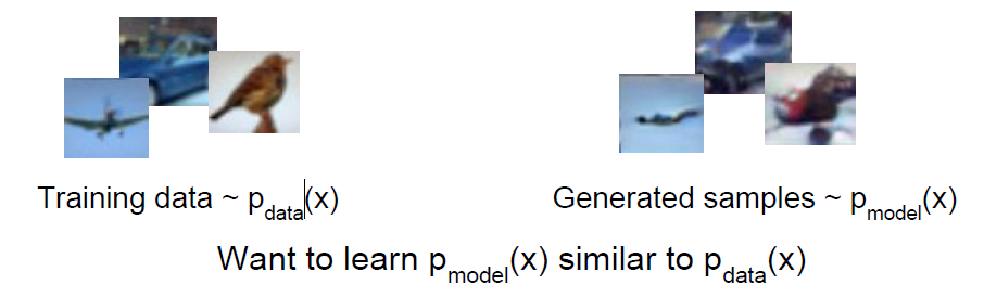
Explicit density estimation or Implicit density estimation.
- Realistic samples for artwork, super-resolution, colorization, etc.
- Generative models of time-series data can be used for simulation and planning (reinforcement learning applications!)
- Training generative models can also enable inference of latent representations that can be useful as general features.
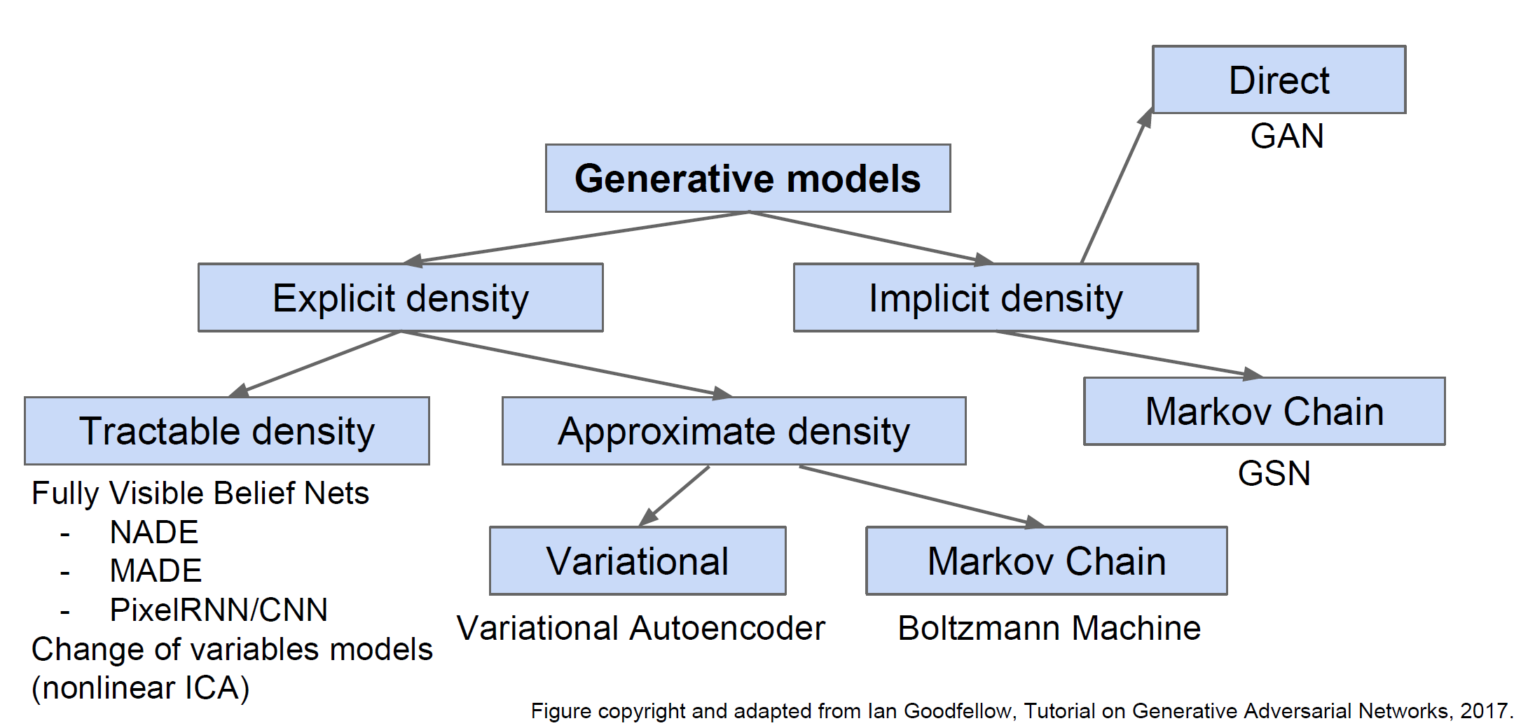
PixelRNN and PixelCNN
Use chain rule to decompose likelihood of an image x into product of 1-d distributions.
\[p(x)=\prod_{i=1}^n p(x_i|x_1,\cdots,x_{i-1})\]$x_i$ means probability of the i pixel value given all previous pixels
Complex distribution over pixel values $\Rightarrow$ Express using a neural
Then maximize likelihood of training data network!
PixelRNN [van der Oord et al. 2016]
Generate image pixels starting from corner. The dependency on previous pixels is modeled using an RNN or LSTM.
Drawback: sequential generation is slow!
PixelCNN [van der Oord et al. 2016]
Still generate image pixels starting from corner
Dependency on previous pixels now modeled using a CNN over context region. We are going to maximize the likelihood if our training data pixels being generated.
Generation must still proceed sequentially so it is still slow.
Autoencoders
Unsupervised approach for learning a lower-dimensional feature representation from unlabeled training data
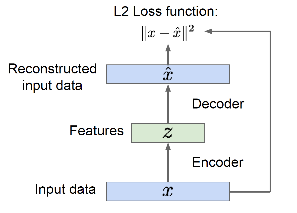
After the training, you can throw away the decoders and using the encoder to initialize a supervised model. Based on this, we were able to use a lot of unlabeled training data to try and learn good general feature representations.
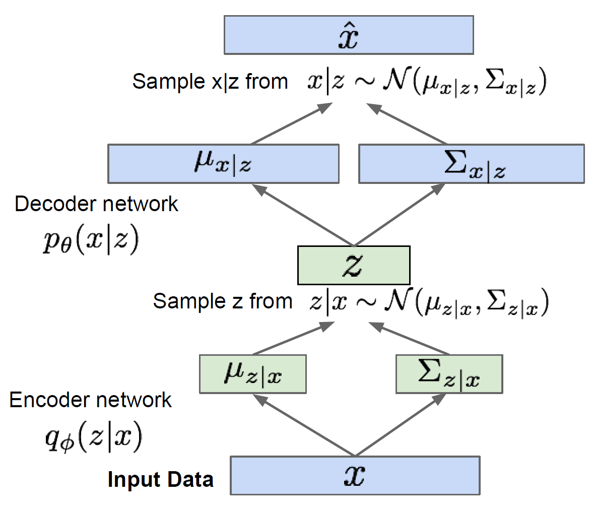
Variational Autoencoders (VAE)
Generative Adversarial Networks (GAN)
GAN will not work on any explicit function, instead, it take a game-theoretic approach.
Instead sample from complex, high-dimensional training distribution, GAN will sample from a simple distribution and learn transformation to training distribution.
Train GANs: Two-player game
- Generator network: try to fool the discriminator by generating real-looking images
- Discriminator network: try to distinguish between real and fake images
$D_{\theta_d}(x)$ is the discriminator output for data x.
$G_{\theta_g}(z)$ is generated fake data from $z$.
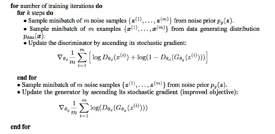
In practice, instead of minimizing likelihood of discriminator being correct, now maximize likelihood of discriminator being wrong, so that we can have a higher gradient signal for bad samples.
GAN training algorithm
Generative Adversarial Nets: Convolutional Architectures [Radford et al, ICLR 2016]

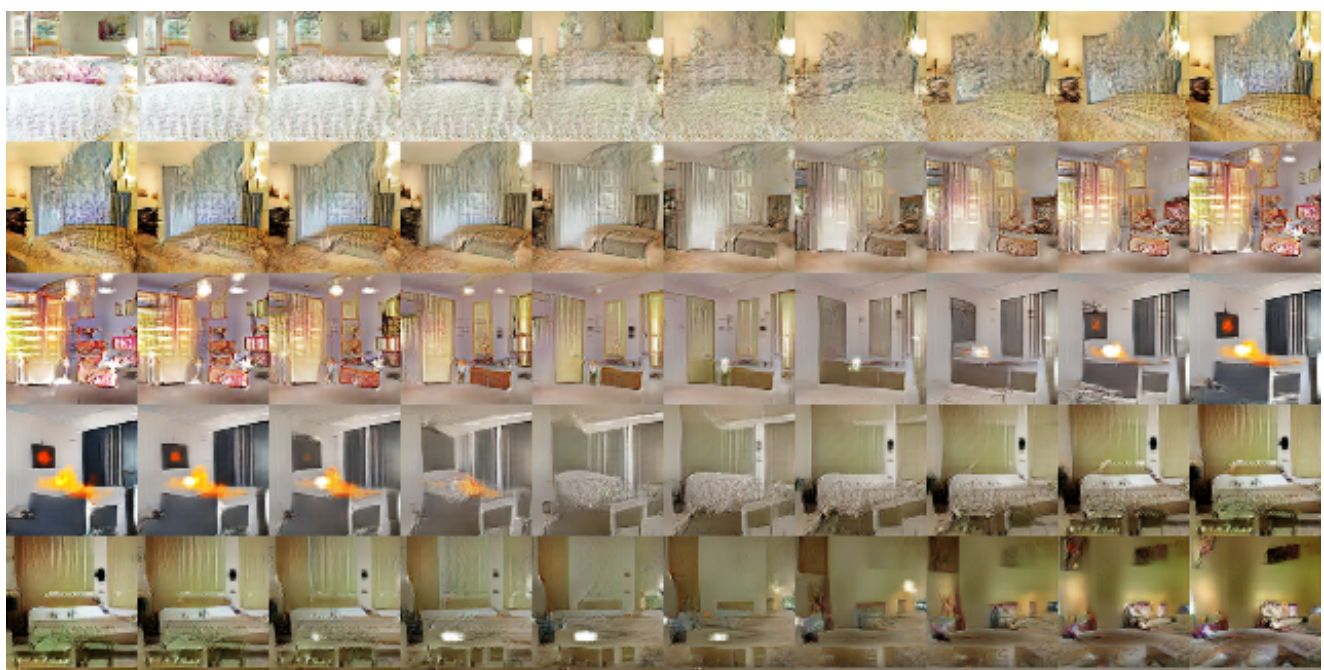
Interpolating between random points in latent space [Radford et al, ICLR 2016]
Also recent work in combinations of these types of models! E.g. Adversarial Autoencoders (Makhanzi 2015) and PixelVAE (Gulrajani 2016)
14. Reinforcement Learning
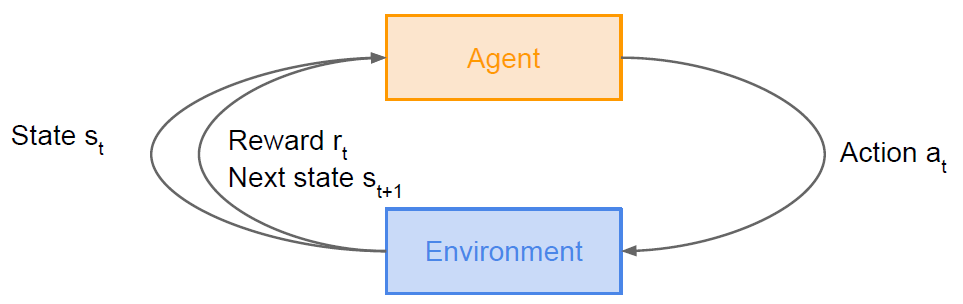
Problems: An agent interacting with an environment,which provides numeric reward signals.
Goal: Learn how to take actions in order to maximize reward
Examples
Cart-Pole Problem
- Objective: Balance a pole on top of a movable cart
- State: angle, angular speed, position, horizontal velocity
- Action: horizontal force applied on the cart
- Reward: 1 at each time step if the pole is upright
Robot Locomotion
- Objective: Make the robot move forward
- State: Angle and position of the joints
- Action: Torques applied on joints
- Reward: 1 at each time step upright + forward movement
Atari Games, Go. etc.
Markov Decision Process
Markov property: Current state completely characterizes the state of the world
A simple MDP: Grid World
Defined by: $(\mathcal{S}, \mathcal{A},\mathcal{R}, \mathbb{P}, \gamma)$
- $\mathcal{S}$: set of possible states
- $\mathcal{A}$: set of possible actions
- $\mathcal{R}$: distribution of reward given (state, action) pair
- $\mathbb{P}$: transition probability i. e. distribution over next state given (state, action) pair
- $\gamma $: discount factor
At time step $t=0$, environment samples initial state $s_0 \sim p(s_0)$
Then, for $t=0$ until done:
- Agent selects action $a_t$
- Environment samples reward $r_t \sim R(\cdot |s_t, a_t)$
- Environment samples next state $s_{t+1} \sim P(\cdot|s_t, a_t)$
- Agent receives reward $r_t$ and next state $s_{t+1}$
A policy $ \pi$ is a function from S to A that specifies what action to take in each state.
Objective: Find policy $\pi^*$ that maximizes cumulative discounted reward $\sum_{t\geq0}\gamma^tr_t$
\[\pi^*=\arg\max_{\pi}\mathbb{E}[\sum_{t\geq0}\gamma^tr_t|\pi] \\ s_0\sim p(s_0),\ a_t\sim \pi(\cdot|s_t),\ s_{t+1}\sim p(\cdot|s_t, a_t)\]Value function
How good is a state?
The value function at state $s$, is the expected cumulative reward from following the policy from state $s$:
\[V^{\pi}(s) = \mathbb{E}[\sum_{t\geq0}\gamma^tr_t|s_0=s,\pi]\]Q-value function
How good is a state-action pair?
The Q-value function at state $s$ and action $a$, is the expected cumulative reward from taking action a in state s and then following the policy.
\[Q^{\pi}(s,a) = \mathbb{E}[\sum_{t\geq0}\gamma^tr_t|s_0=s,a_0=a,\pi]\]Bellman equation
The optimal Q-value function $Q^*$ is the maximum expected cumulative reward achievable from a given (state, action) pair:
\[Q^{*}(s,a) = \max_\pi\mathbb{E}[\sum_{t\geq0}\gamma^tr_t|s_0=s,a_0=a,\pi]\]$Q^*$ satisfies the following Bellman equation:
\[Q^*(s,a) = \mathbb{E}_{s'}\sim\epsilon[r+\gamma\max_{a'}Q^*(s',a')|s,a]\]The optimal policy $\pi^$ corresponds to taking the best action in any state as specified by $Q^$.
Value iteration algorithm: Use Bellman equation as an iterative update
\[Q_{i+1}(s,a) = \mathbb{E}[r+\gamma\max_{a'}Q_i(s',a')|s,a]\]$Q_i$ will converge to $Q^*$ as $i\rightarrow\inf$. However, it is not scalable because we must compute Q(s,a) for every state-action pair. If state is so much, computationally infeasible to compute for entire state space! This inspires us to using a function approximator to estimate Q(s,a), such as a neural network!
Q-Learning
Use a function approximator to estimate the action-value function. If the function approximator is a deep neural network, it will be called deep Q-learning.
\[Q^*(s,a) = \mathbb{E}_{s'}\sim\epsilon [r+\gamma\max_{a'}Q^*(s',a')|s,a]\]Forward Pass
\[L_i(\theta_i) = \mathbb{E}_{s,a\sim\rho(\cdot)}[(y_i-Q(s,a;\theta_i))^2]\] \[y_i=\mathbb{E}_{s'}\sim\epsilon [r+\gamma\max_{a'}Q^*(s',a';\theta_{i-1})|s,a]\]Backward Pass
\[\nabla_{\theta_i}L_i(\theta_i)=\mathbb{E}_{s,a\sim\rho(\cdot);s'}\sim\epsilon[r+\gamma\max_{a'}Q(s',a';\theta_{i=1})-Q(s,a;\theta_i)\nabla_{\theta_i}Q(s,a;\theta_i)]\]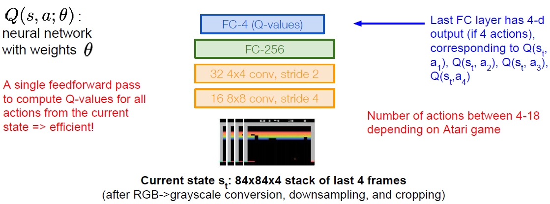
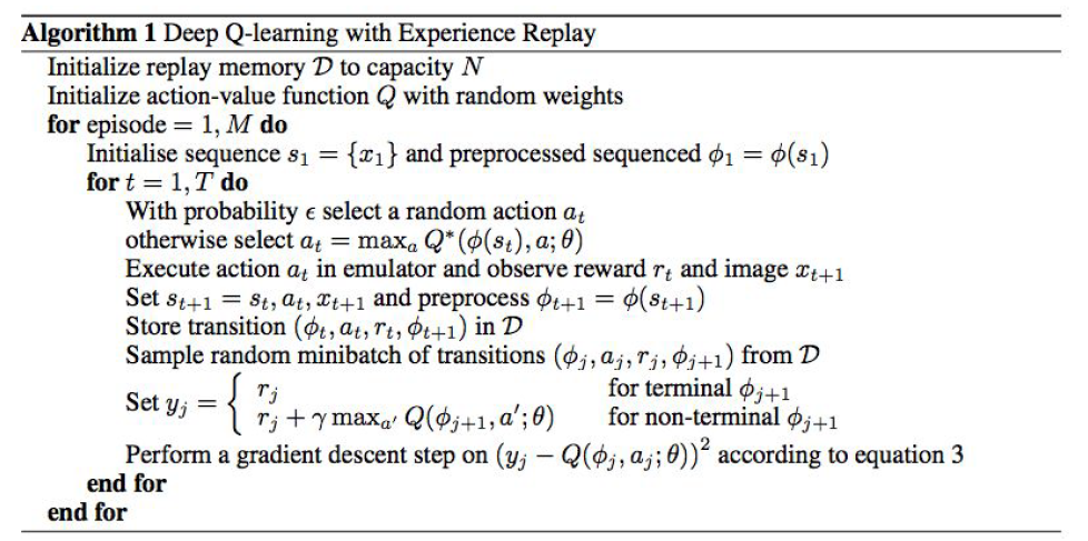
Training the Q-network: Experience Replay
-
Continually update a replay memory table of transitions ($s_t, a_t, r_t, s_{t+1}$) as game (experience) episodes are played
-
Train Q-network on random minibatches of transitions from the replay memory, instead of consecutive samples
Policy Gradients
Let’s define a class of parametrized policies: $\Pi={\pi_\theta, \theta\in\mathbb{R}^m}$
For each policy,define its value: $J(\theta)=\mathbb{E}[\sum_{t\ge0}\gamma^tr_t|\pi_\theta]$, we can use gradient ascent on policy parameters to find the optimal policy $\theta^*=\mathbb{E}[\sum_{t\geq0}\gamma^tr_t|\pi_\theta]$ .
We have:
\[J(\theta)=\mathbb{E}_{\tau\sim p(\tau;\theta)}[r(\tau)]=\int_\tau r(\tau)p(\tau;\theta)d\tau\]where $r(\tau)$ is the reward of a trajectory $\tau=(s_0, a_0, r_0,s_1,\cdots)$
Now we can derive the gradient with the respect to $\theta$:
\[\nabla_\theta J(\theta)=\int_\tau r(\tau)\nabla_\theta p(\tau;\theta)d\tau \\\nabla_\theta p(\tau;\theta)=p(\tau;\theta)\frac{\nabla_\theta p(\tau;\theta)}{p(\tau;\theta)}=p(\tau;\theta)\nabla_\theta \log p(\tau;\theta)\]So we have:
\[\nabla_\theta J(\theta)=\int_\tau (r(\tau)\nabla_\theta\log p(\tau;\theta))p(\tau;\theta)d\tau =\mathbb{E}_{\tau\sim p(\tau;\theta)}[r(\tau)\nabla_\theta\log p(\tau;\theta)] \\\log p(\tau;\theta)=\sum_{t\geq0}\log p(s_{t+1}|s_t, a_t) + \log \pi_{\theta}(a_t|s_t) \\\nabla_\theta J(\theta)\approx\frac{1}{N}\sum_{i=1}^N(r(\tau_i)\sum_{t\geq0}\nabla_\theta\log\pi_\theta(a_t|s_t))\]This means we can estimate this expectation using Monte Carlo sampling.
Variance reduction
- Push up probabilities of an action seen, only by the cumulative future reward from that state.
- Use discount factor $\gamma$ to ignore delayed effects.
- Introduce a baseline function dependent on the state. We want to push up the probability of an action from a state, if this action was better than the expected value of what we should get from that state.
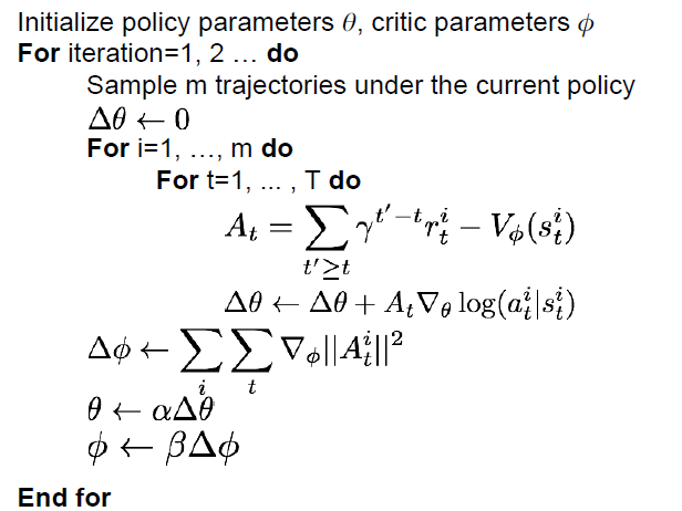
Actor-Critic Algorithm
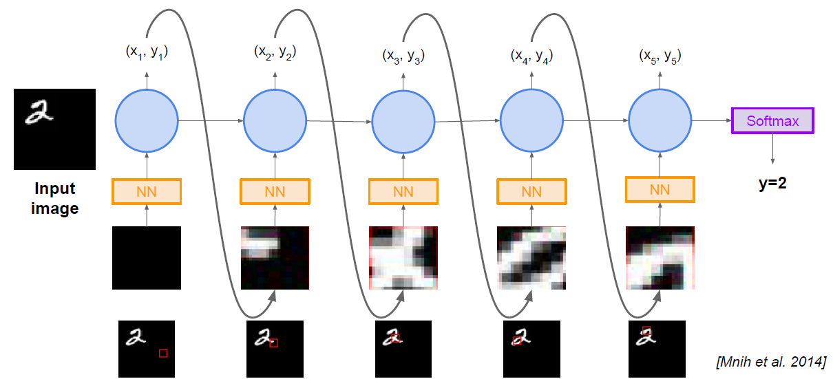
Reinforce in action: Recurrent Attention Model (RAM) [Mnih et al. 2014]
AlphaGo [Silver et al., Nature 2016]
15. Efficient Methods and Hardware for Deep Learning
Challenge: Model size, speed, energy efficiency
Improve the Efficiency of Deep Learning by Algorithm-Hardware Co-Design
Hardware family: General Purpose/Specialized Hardware
- General Purpose: CPU: latency oriented and single threaded
- GPU: throughout oriented
- Specialized Hardware: FPGA: field programmable gate array
- ASIC: application specific integrated circuit, fixed logic
Number Representation
\[(-1)^s\times (1.M)\times 2^E\]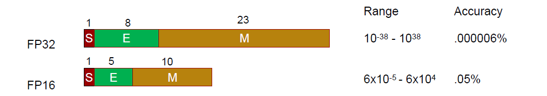
Going from 32bit to 16bit, we have about four times reduction in energy and area.
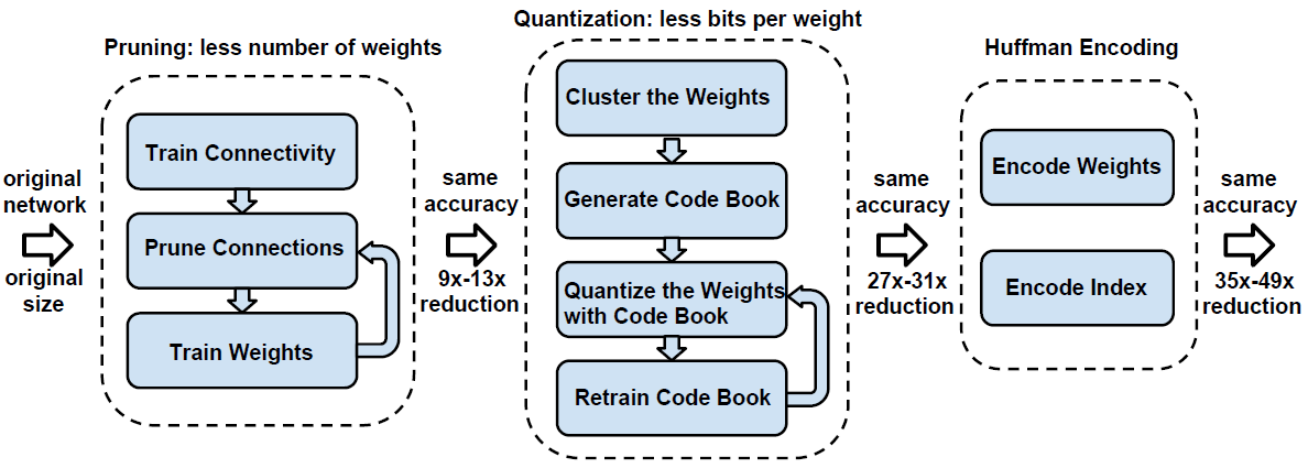
Pruning Neural Networks
Remove some of the weights and get rid of those redundant connections, but we can still keep the accuracy.
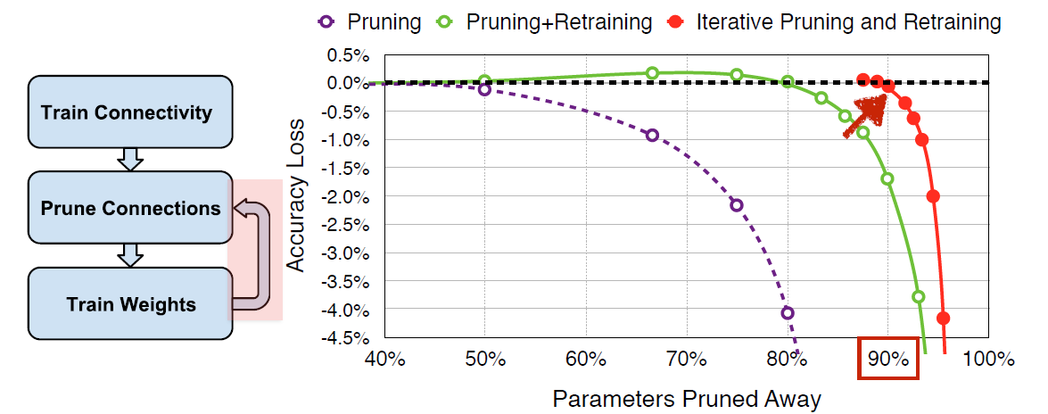
If we do this process iteratively by pruning and retraining, we can fully recover the accuracy not until we are prune away 90% of the parameters.
Weight Sharing
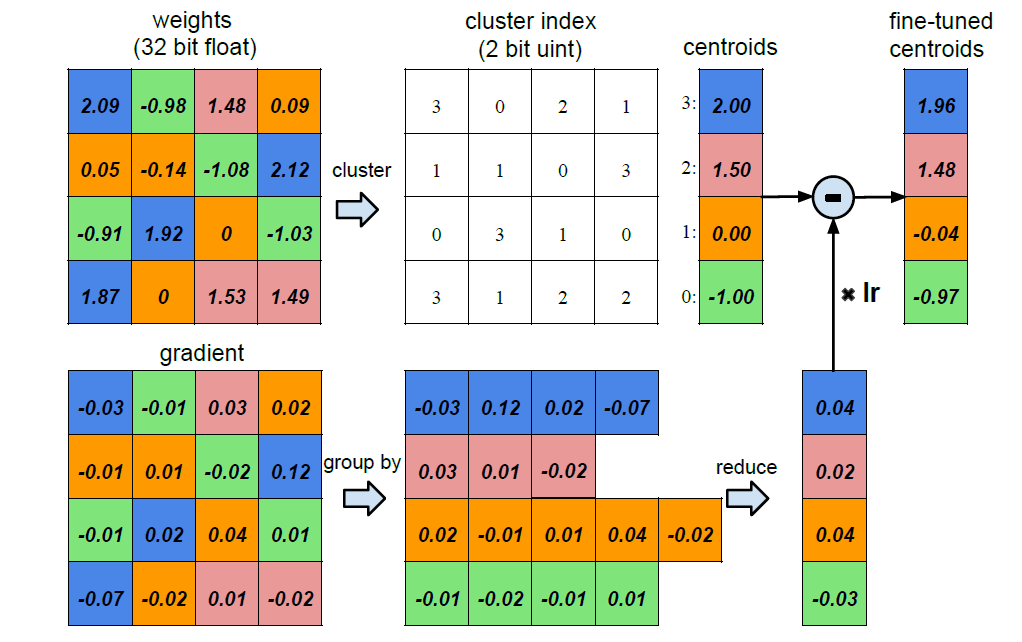
We do k-means clustering by having the similar weight sharing the same centroid. So that we only need to store the two bit index rather than 32 bit floating point number.
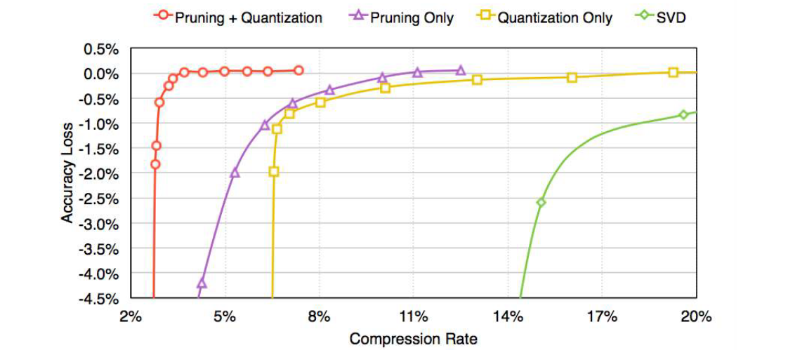
If we combine these two methods together, we can make the model about 3% of its original size without hurting the accuracy at all.
So now we consider that can we begin with a compact model, and the answer is true.
SqueezeNet: AlexNet-level accuracy with 50x fewer parameters and< 0.5 MB model size.
And note that we can still do compression on this net to get 510 ratios smaller than the AlexNet but similar accuracy.
Quantization
-
Train with float
-
Quantizing the weight and activation: Gather the statistics for weight and activation and choose proper radix point position
-
Fine-tune in float format and convert to fixed-point format
Low rand approximation
For a convolution layer, you can break it into two convolution layers. For example, you can decompose a convolution layer with $d$ filters with filter size $k\times k\times c$ to:
- A layer with $d’$ filters $(k\times k\times c)$
- A layer with $d$ filters $(1\times 1\times d’)$
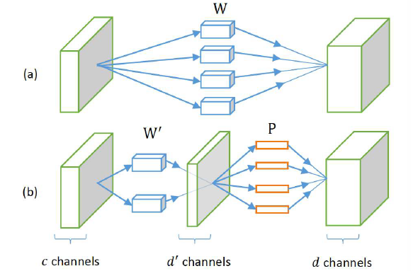
Achieving about 2x speed up, there’s almost no loss of accuracy.
For fully connected layers, we can use tensor tree to break down one layer into lots of fully connected layers using SVD method.
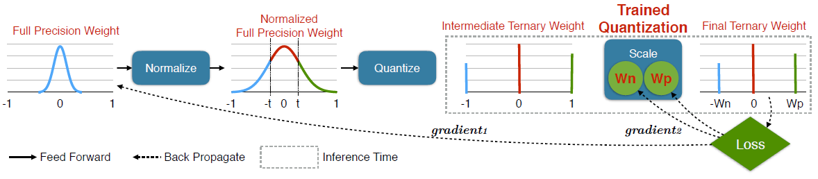
Binary or Ternary Net
We maintain a full precision weight during training time, but at inference time, we only keep the scaling factor and the ternary weight.
Winograd Transformation
“Fast algorithms for convolutional neural networks.” Proceedings of the IEEE Conference on Computer Vision and Pattern Recognition. 2016
After cuDNN5, the cuDNN begins to use the Winograd Transformation.
Hardware for Efficient Inference
Google TPU
We need hardware that can infer on compressed model. So we have EIE: the efficient inference engine, which deals with those sparse and compressed model to save the memory bandwidth.
We can only save and run the calculation on the non-zero parameters. And using such efficient hardware architecture and model compression, we can get a better efficiency and speed than CPU, GPU or ASIC.
Parallelization
As the time goes by, for the number of transistors on CPU is keeping increasing, but the single threaded performance and the frequency are getting plateaued in recent yeas because the power constraint. However, the number of cores is increasing.
Data parallel: Run multiple training examples in parallel
Model parallel: Split model over multiple processors by layer or conv layers by map region or fully connected layers by output activation
Hyper-parameter parallel
Mixed Precision with FP16 and FP32
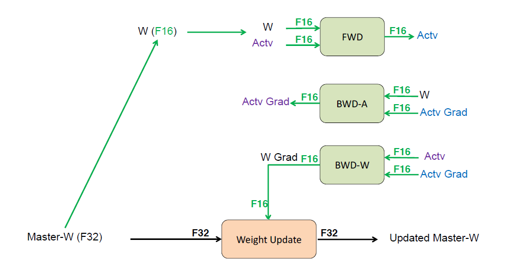
Mixed precision training. arXiv preprint arXiv:1710.03740 (2017).
Model Distillation
Use multiple large powerful senior neural network to teach the student model, which has much smaller model size.
Hinton, Geoffrey, Oriol Vinyals, and Jeff Dean. “Distilling the knowledge in a neural network.” arXiv preprint arXiv:1503.02531 (2015).
DSD: Dense-Sparse-Dense Training
DSD produces same model architecture but can find better optimization solution, arrives at better local minima, and achieves higher prediction accuracy across a wide range of deep neural networks on CNN/ RNN / LSTM.
Han, Song, et al. “DSD: Dense-sparse-dense training for deep neural networks.” arXiv preprint arXiv:1607.04381 (2016).
Hardware for Efficient Training
- New in Volta: Tensor Core
- Google Cloud TPU
16. Adversarial Examples and Adversarial Training
- What are adversarial examples and why do they happen?
- How can they be used to compromise machine learning systems?
- What are the defenses and how to use adversarial examples to improve machine learning?
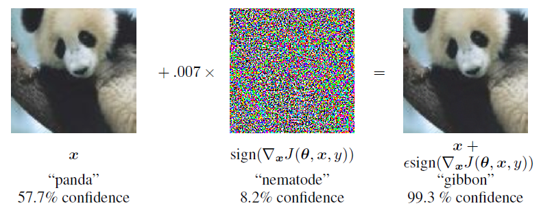
An adversarial example is an example that has been carefully computed to be misclassified. In a lot of cases we are able to make the new image indistinguishable to a human observer from the original image.
It is important to remember that these vulnerabilities apply to essentially every machine learning algorithm that we have studied so far. Some of them like RBF networks and partisan density estimators are able to resist this effect somewhat, but even very simple machine learning algorithms are highly vulnerable to adversarial examples, including Logistic regression and SVM.
It was found that many different models would mis-classify the same adversarial examples, and they would sign the same class to them. And it was also found that if we took the difference between an original example and an adversarial example, then we had a direction in input space. We could add that same offset vector to any clean example, and we would almost always get an adversarial example as a result.
Early attempts at explaining this phenomenon focused on nonlinearity and overfitting. We argue instead that the primary cause of neural networks’ vulnerability to adversarial perturbation is their linear nature. This explanation is supported by new quantitative results while giving the first explanation of the most intriguing fact about them: their generalization across architectures and training sets.
Modern deep networks are very piecewise linear rather than being a single linear function.
The mapping from the input to the output is much more linear and predictable, which means that optimization problems that aim to optimize the input to the model are much easier than optimization problems that aim to optimize the parameters.
We are able to get quite a large perturbation without changing the image very much as far as a human being is concerned. Here all three perturbations have L2 norm 3.96.
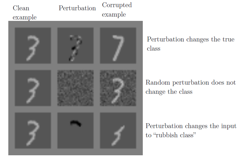
Actually a lot of the time with adversarial examples, you make perturbations that have an even larger L2 norm. What’s going on is that there are several different pixels in the image, and so small changes to individual pixels can add up to relatively large vectors. For larger datasets like ImageNet, where there is more pixels, you can make very small changes to each pixel that travel very far in vector space as measured by L2 norm. That means you can actually make changes that are almost imperceptible but actually move you really far and get a large dot product with the coefficients of the linear function that the model represents.
The Fast Gradient Sign Method
\[J(\tilde{x}, \theta) \approx J(x,\theta) + (\tilde x - x)^T\nabla_xJ(x)\] \[max \hspace{1cm} J(x,\theta) + (\tilde x - x)^T\nabla_xJ(x) \\ s.t. \hspace{1cm} ||\tilde x-x||_{\infty}\leq\epsilon\] \[\Rightarrow \tilde x = x + sign(\nabla_xJ(x)) \times \epsilon\]The maps of adversarial and random cross-sections
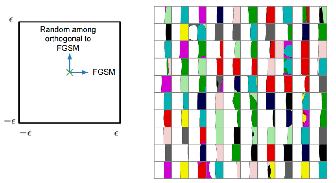
Note that for the most part, the noise has very little effect on the classification decision compared to adversarial examples. Because if you choose some reference vector in some high dimensional spaces, and then you choose a random vector in that space, the random vector will, on average, have zero dot product with the reference vector.
The dimensionality of the subspace where the adversarial examples lie in actually tells you something about how likely you are to find an adversarial example by generating random noise. The average dimensionality on MINIST dataset is 25.
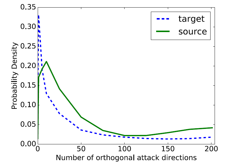
Different models will often mis-classify the same adversarial examples. The larger the dimensionality of the subspace, the more likely it is that the subspaces for two models will intersect.
If we look at the percentage of the space in RN that is correctly classified, we find that they mis-classify almost everything, and they behave reasonably only on a very thin manifold surrounding the data that we train them on.
Right now, adversarial examples for reinforcement learning are very good at showing that we can make reinforcement learning agents fail. But we haven’t yet been able to hijack them and make them do a complicated task that’s different from what their owner intended. Seems like it’s one of the next steps in adversarial example research though.
Some quadratic models actually perform really well. In particular a shallow RBF network is able to resist adversarial perturbations very well. Because the model is so nonlinear and has such wide flat areas that the adversary is not able to push the cost uphill just by making small changes to the model’s input.
Transferability Attack
cross technique transferability
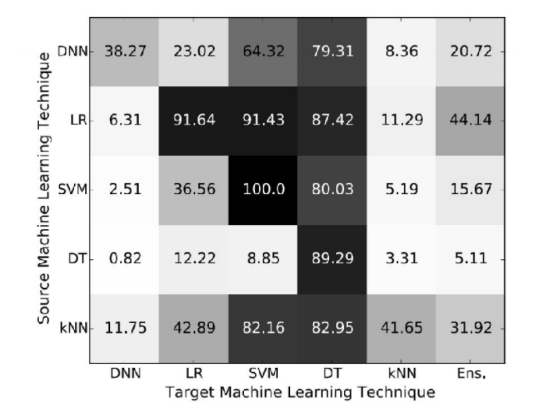
If the target model with unknown weights, machine learning algorithms and even train set, they can train their own model to do the attack. There is two different way, one is you can label your own training set for the same task that you want to attack. And the other is that you can send inputs to the model and observe its outputs, then use those as your training set. This will work even if the output that you get from the target model is only the class label that it chooses.
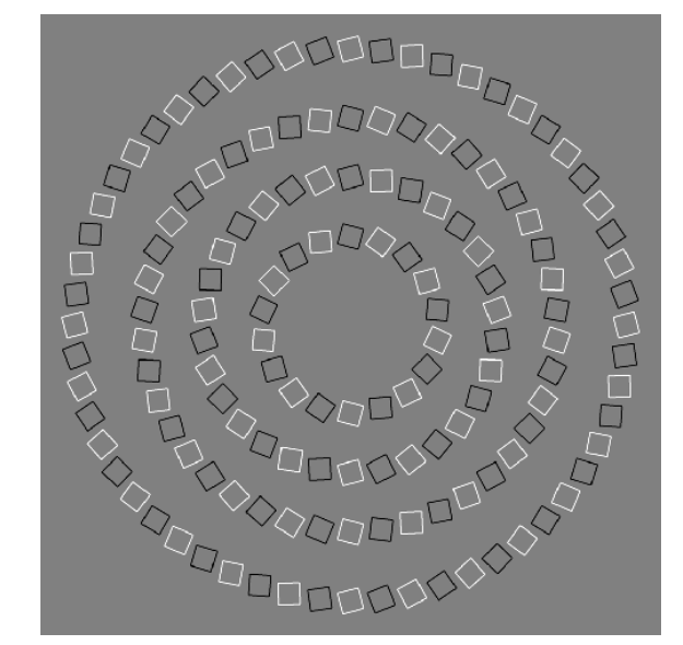
Adversarial Examples in the Human Brain
Studying adversarial examples tells us how to significantly improve our existing machine learning models.
Practical Attack
- Fool real classifiers trained by remotely hosted API (MetaMind, Amazon, Google)
- Fool malware detector networks
- Display adversarial examples in the physical world and fool machine learning systems that perceive them through a camera (Kurakin et al, 2016)
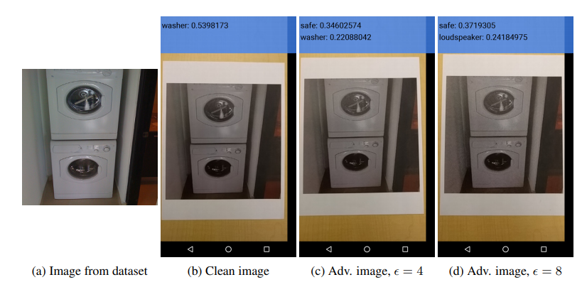
The attacker could conceivably fool a system that’s deployed in a physical agent, even if they don’t have access to the model on that agent and even if they can’t interface directly with th agent but just modify objects that it can see in its environment.
Training on Adversarial Examples
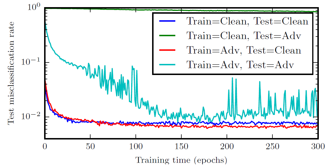
Adversarial trained neural nets have the best empirical success rate on adversarial examples of any machine learning model. SVM or linear regression cannot learn a step function, so adversarial training is less useful, very similar to weight decay.
However, even with adversarial training, we are still very far from solving this problem.
Virtual Adversarial Training and semi-supervised learning
Universal engineering machine (model-based optimization)
If we are able to do model-based optimization, then we can write a function that describes a thing that doesn’t exist yet but we wish that we had, which means we can make new inventions by finding input that maximizes model’s predicted performance.